rcisignal: User's Guide

Last updated: 07-06-2026

1. Overview

rcisignal is a toolkit for examining the data quality of reverse-correlation (RC) experiments and for triangulating any signal captured in the dataset (e.g., a hypothesized mental representation of a friendly face). It addresses three questions, in order. First, are the inputs clean (response coding, trial counts, response bias, stimulus-pool alignment)? Second, is the signal informative and stable (does each condition’s group CI carry more pattern than chance, and would the pattern replicate on a different half of the producers)? Third, when there is more than one condition, are the conditions distinguishable, both in overall magnitude and in spatial location?

Two halves of the package address these questions in turn. The input-side diagnostics (run_diagnostics() and the check_* family, plus infoval_report() for the focused “is my data informative at all?” summary) cover the first question. The output-side reliability and discriminability metrics (run_reliability(), run_discriminability(), infoval(), agreement_map_test(), together with the lower-level building blocks rel_*() and pixel_t_test()) cover the second and third.

1.1 Scope

For 2IFC stimulus generation and CI computation, rcisignal delegates to the upstream rcicr package (Dotsch, 2016, 2023). ci_from_responses_2ifc() is a small convenience function around rcicr::batchGenerateCI2IFC() that takes care of the integration quirks. Brief-RC support (Schmitz, Rougier, & Yzerbyt, 2024) is provided directly by rcisignal via ci_from_responses_briefrc().

The metrics in this package quantify whether a CI is stable (within-condition) and separable (between-condition). Whether the CI accurately reflects the producer’s mental representation of the target trait is a separate validity question, typically addressed by an external rater study, and sits outside the package. Cone, Brown-Iannuzzi, Lei, & Dotsch (2021) showed that the standard two-phase rating design inflates Type I error; rcisignal’s metrics operate directly on producer-level pixel signal and thereby sidestep that pitfall.

The intended audience is RC researchers at an intermediate R level with basic familiarity with the rcicr package or with the Schmitz et al. (2024) Brief-RC structure. No prior expertise in data.table, permutation testing, or intraclass correlation is assumed.

1.2 Validation status

Worth flagging before any published use of this package: not all of the metrics it ships are independently validated for social-face RC data. The package is best treated as a toolbox that collects existing methods, plus a few natural extensions of those methods, into one place. Some of those extensions are mature and well-grounded in adjacent literatures; others are sensible-looking implementations that have not yet had a dedicated validation study on the kind of data this package targets. Reporting accordingly matters.

Validated in their respective domains:

• Per-producer infoVal for 2IFC (Brinkman et al., 2019). The Frobenius-norm magnitude statistic, its modified-z formulation against a random-responder reference distribution, and the Type-I/power validation on social-face 2IFC data all originate from the Brinkman et al. paper. (The reporting threshold itself, z >= 1.96, is the conventional standard-normal cutoff that Brinkman et al. adopt: a one-sided 2.5%, equivalently two-sided 5%, error rate.)
• Pixel-test methodology (Chauvin et al., 2005). The per-pixel inferential test on smooth classification images — and the cluster-level companion — are well-established in the classification-image and neuroimaging literatures. Chauvin et al. use a per-pixel Z-statistic on the noise-response correlation calibrated by Random Field Theory; rcisignal adapts the same logic to the per-producer signal matrix and calibrates instead by sign-flip permutation (see §12.1).
• Cluster-based permutation tests for FWER control (Maris & Oostenveld, 2007). Validated on EEG and MEG data, with the underlying logic carrying over to any spatial statistical map.
• Threshold-free cluster enhancement (TFCE) (Smith & Nichols, 2009). Validated on neuroimaging data; same transferability caveat as above.

Package-level extensions, not yet independently validated for face evaluation RC:

• Group-mean infoVal. A natural extension of per-producer infoVal to the group-average CI, with a trial-count-matched reference. Brinkman et al. (2019) recommend reporting the distribution of per-producer infoVals rather than a single group z; the group-mean version is offered here as a supplementary summary, not as a replacement for the per- producer reporting. See §11 for the full description, how the matched-N reference distribution is constructed, and a calibration illustration.
• Between-condition discriminability tests (cluster-based permutation and TFCE). The underlying machinery is borrowed from neuroimaging where it is well-validated; its specific behavior on social-face CI maps (which differ from EEG/MEG or fMRI in spatial structure, signal-to-noise, and base-image artefacts) has not been the subject of a dedicated validation study.
• Pixel-wise agreement / reliability maps (agreement_map_test() and the related plot helpers). Same machinery as above, applied within a single condition. Same caveat.
• infoVal applied to Brief-RC. The Frobenius-norm logic transfers, and the trial-count-matched reference closes the most obvious calibration gap relative to a pool-keyed reference. The threshold conventions inherited from 2IFC have not been re-validated on Brief-RC.

If you use the unvalidated metrics in published work, please report them as exploratory and indicate the package version. If you are aware of validation studies I have missed, I would be glad to update this section (m.j.barbosa.de.oliveira@tue.nl).

For the engine-equivalence receipts behind the per-producer 2IFC infoVal claim above (and a Brief-RC signal-recovery sanity check), see vignette("validation_rcicr", package = "rcisignal").

1.3 Per-producer CIs and the optional group_by = shortcut

ci_from_responses_briefrc() and ci_from_responses_2ifc() produce a $signal_matrix of pixels x n_producers (one column per producer). Every reliability, discriminability, and informational- value function in the package takes this object as its primary input: infoval(), rel_split_half(), rel_icc(), rel_loo(), rel_cluster_test(), rel_dissimilarity(), agreement_map_test(), pixel_t_test(), plus the three run_* orchestrators.

cis <- ci_from_responses_briefrc(responses,
                                 noise_matrix = noise_matrix)
cis$signal_matrix          # pixels x n_producers
run_reliability(cis$signal_matrix, n_permutations = 200L)
infoval(cis$signal_matrix, noise_matrix,
        responses = responses, iter = 500L)

When you want CIs averaged by condition (or another grouping column), the cheapest way is to pass group_by = to the generator and read both matrices off the same return list:

# `group_by` names a column (or columns) in `responses`. The
# generator calls `group_ci()` for you and returns both matrices
# on the same return list.
res <- ci_from_responses_briefrc(
  responses, noise_matrix = noise_matrix, group_by = "condition"
)
res$signal_matrix          # pixels x n_producers (as before)
res$group_ci               # pixels x n_groups (one column per condition)

group_ci() is also exported as a standalone helper. Use it when you already have a per-producer signal matrix in hand (eg one read back from disk) and want to collapse producers into per-group means with the same validation (each producer’s by value(s) must be constant across their rows; producers in colnames(signal_matrix) must be present in responses).

Once you have $group_ci, the per-condition CIs sit in one matrix and are ready to be compared. The package ships three plot functions for asking how similar the group CIs are to each other: plot_ci_distance_matrix() for all-vs-all Euclidean distance, plot_ci_correlogram() for pairwise Pearson r, and plot_ci_mds() for a 2D map of the same distances. All three accept any named collection of CIs (per-producer or group-level), so the same call works on $signal_matrix, $group_ci, a named matrix built with cbind(), or a named list. Column names become the labels in the figure.

# How distinct are the per-condition CIs from each other?
plot_ci_distance_matrix(res$group_ci)

1.4 Exporting CIs as PNG or JPEG

save_ci_images() writes each column of a signal matrix to disk as its own image. The same call works for per-producer matrices and for group-averaged matrices; the function picks a sensible filename prefix based on what you hand it.

out_dir <- tempfile("oliveira_cis_"); dir.create(out_dir)

# One PNG per producer: ind_ci_P001.png, ind_ci_P002.png, ...
save_ci_images(res$signal_matrix, base_image = sim$base_face,
               dir = out_dir)

# One PNG per condition: group_ci_A.png, group_ci_B.png, ...
save_ci_images(res$group_ci, base_image = sim$base_face,
               dir = out_dir)

The default output is a grayscale luminance image that matches what rcicr::generateCI() / rcicr::generateCI2IFC() would write for the same CI: the raw signed noise is scaled into [0, 1] via the chosen scaling method (default "independent", matching rcicr’s default) and then averaged with the base via (scaled + base) / 2. No color palette is involved. The four scaling options ("independent", "constant", "matched", "none") and the scaling_constant argument are the rcicr ones, with the same meanings.

Two color palettes are available as opt-ins for visualization: palette = "diverging" (signed CI on the same blue/red ramp plot_ci_overlay() uses) and palette = "fire" (unipolar |t|-style yellow-to-red). Pass format = "jpeg" to write JPEGs instead, or prefix = "trust_" (or any other string) to override the auto-derived filename prefix.

2. Installation

# Latest release from GitHub.
remotes::install_github("olivethree/rcisignal",
                        dependencies = TRUE)

# rcicr is a Suggests dep; install it if you need the 2IFC path.
install.packages("rcicr")               # CRAN
remotes::install_github("rdotsch/rcicr") # development

The mandatory dependencies are minimal (cli and data.table, plus the base packages). PNG and JPEG readers (png, jpeg), rcicr for 2IFC pipelines, and psych for ICC cross-validation sit in Suggests and load on demand.

rcisignal is in an experimental stage and exported functions are still being refined. Re-running the install_github() call above at the start of each analysis session pulls the latest version; this user guide is kept in sync with new and updated functions.

library(rcisignal)

2.1 Quickstart with simulated data

Two helpers, simulate_2ifc_data() and simulate_briefrc_data(), generate a complete synthetic dataset (responses + noise pool +, for 2IFC, an rcicr-format .Rdata) so the rest of this vignette can be exercised without needing to bring your own files. They are also building blocks for simulation studies (power, calibration of reliability and discriminability metrics, sensitivity to contamination).

What they generate

• Responses. A long-format data.table with one row per trial and the columns every diagnostic / CI function expects: participant_id, condition, trial, stimulus, response (in {-1, +1}), rt (in milliseconds).
• Noise pool. A pixels x n_trials numeric matrix, generated on the fly via rcicr::generateNoisePattern() and rcicr::generateNoiseImage(). (rcicr must be installed; with the default 256-pixel images and 500 trials the pool takes roughly one to three minutes, with a cli progress bar.)
• For 2IFC, an .Rdata file in the format that rcicr::generateStimuli2IFC() writes, so ci_from_responses_2ifc(), infoval_report(), and every other function that asks for an rdata argument works out of the box.
• A self-contained $stimuli list that round-trips through saveRDS()/readRDS() and a $base_image_path PNG written next to the stimuli .Rdata. The first survives session restarts when handed to a consumer via stimuli =; the second is the rcicr-style on-disk artefact for tools that expect a base-face file.

The return value is an rcisignal_sim S3 object:

sim <- simulate_2ifc_data()
str(sim, max.level = 1)
#> List of 10
#>  $ data            : data.table  [50000 x 6]
#>  $ noise_matrix    : num [1:65536, 1:500]   (pixels x trials)
#>  $ base_face       : num [1:256, 1:256]
#>  $ params          : num [1:500, 1:4092]    (rcicr stimuli_params)
#>  $ p               : list of 4               (rcicr noise basis)
#>  $ signal          : num [1:65536]           (planted signal vector)
#>  $ rdata_path      : chr "/tmp/.../rcisignal_sim_2ifc_stimuli.Rdata"
#>  $ base_image_path : chr "/tmp/.../rcisignal_sim_2ifc_base_face.png"
#>  $ stimuli         : list of 11             (portable, round-trips via saveRDS)
#>  $ meta            : list (seed, elapsed, etc.)

Defaults

Argument	Default	Notes
n_per_condition	50	participants per condition
conditions	c("target", "control")	any character vector works
n_trials	500 (2IFC); NULL (Brief-RC)	per participant; equals the noise pool size for 2IFC. For Brief-RC, NULL derives it from noise_pool_size
images_per_trial (Brief-RC only)	12	= 6 original/inverted pairs
noise_pool_size (Brief-RC only)	500	shared across participants; if n_trials is given instead, it is n_trials * (images_per_trial / 2)
img_size	256	pixels; matches the bundled base face
base_image	inst/extdata/sim_base_face.png	a 256x256 grayscale artificial face; pass a path or matrix to override
signal_strength	"weak"	also "none" (true null), "strong", or a numeric coefficient
signal_region	"eyes"	any region accepted by make_face_mask()
rt_contamination_fast / _slow	0.02 / 0.02	fraction of trials replaced by uniform-fast (50-200 ms) / uniform-slow (5000-20000 ms) responses
noise_type, nscales, sigma	"sinusoid", 5, 25	forwarded to rcicr::generateNoisePattern()
rdata_dir	NULL	optional directory for a stable-path stimuli .Rdata; pass to keep the sim usable across R sessions
seed	NULL	a random seed is drawn and stored on the result
progress	TRUE	shows a cli progress bar during noise generation

Signal model

Each trial’s response is drawn from a logistic / softmax model whose location depends on a planted pixel-level signal s (the binary mask returned by make_face_mask() for the chosen signal_region).

• 2IFC. On each trial t the participant sees image_a = base + noise[t] and image_b = base - noise[t] and chooses one. The log-odds of choosing image_a (response = +1) are beta * (noise[, t] %*% s) / sqrt(sum(s)). With signal_strength = "none" (beta = 0), choices are uniform random; with "weak" (beta = 0.5) the planted region biases responses just enough that a 50 x 2 x 500 dataset yields a recognisable cluster on the eyes region; "strong" (beta = 2) produces a much sharper signal.
• Brief-RC. Each trial shows images_per_trial = 2k images (the original and inverted versions of k distinct noise patterns drawn from the shared pool). Each image gets a Gumbel-perturbed utility ±beta * (noise %*% s) / sqrt(sum(s)) + Gumbel(0,1) and the participant picks the argmax (multinomial-logit / softmax). The recorded stimulus is the pool index of the chosen pair; response is +1 if the original version of that pair was chosen, -1 if the inverted version.

A weak signal is the default rather than "none" so the worked example produces a recognisable CI on the planted region rather than a flat null result. Pass signal_strength = "none" to get truly bogus data (useful for testing the diagnostic side, calibrating null distributions, or stress-testing the reliability / cluster permutation code under no-signal conditions).

Response-time model

RTs follow a shifted lognormal (rt = round(exp(rnorm(n, log(800), 0.5)) + 150), in milliseconds) with two contaminant streams:

• Fast contaminants at rt_contamination_fast (default 2%): uniform [50, 200] ms, mimicking accidental clicks.
• Slow contaminants at rt_contamination_slow (default 2%): uniform [5000, 20000] ms, mimicking distraction or task pauses.

These are deliberately tuned so that check_rt() finds something to flag (useful for sanity-checking the RT diagnostic without curating real outliers by hand).

End-to-end demo (2IFC)

Pasting the chunk below into a fresh R session takes you from no data at all to a within-condition reliability summary:

sim <- simulate_2ifc_data(
  n_per_condition = 30,    # smaller for a quick demo
  n_trials        = 200,
  signal_strength = "weak",
  seed            = 1
)

# Step 1: run the diagnostic battery on the simulated responses.
# Pass the simulator's rdata so rdata-dependent sub-checks (response
# inversion, infoval consistency) run too. `stimuli = sim$stimuli`
# is an in-memory equivalent.
print(run_diagnostics(sim$data, method = "2ifc",
                      rdata = sim$rdata_path, col_rt = "rt"))

# Step 2: compute per-participant CIs using the bundled .Rdata.
target_rows  <- subset(sim$data, condition == "target")
control_rows <- subset(sim$data, condition == "control")
cis_target   <- ci_from_responses_2ifc(target_rows,
                                       rdata_path = sim$rdata_path)
cis_control  <- ci_from_responses_2ifc(control_rows,
                                       rdata_path = sim$rdata_path)

# Step 3: within-condition reliability.
print(run_reliability(cis_target$signal_matrix,  seed = 1))
print(run_reliability(cis_control$signal_matrix, seed = 1))

# Step 4: between-condition cluster test.
print(run_discriminability(
  signal_matrix_a = cis_target$signal_matrix,
  signal_matrix_b = cis_control$signal_matrix,
  seed            = 1
))

For the Brief-RC pipeline the equivalent demo replaces simulate_2ifc_data() with simulate_briefrc_data() and ci_from_responses_2ifc() with ci_from_responses_briefrc(). The Brief-RC consumer reads the noise matrix directly, so the call becomes ci_from_responses_briefrc(sim$data, noise_matrix = sim$noise_matrix); add base_image = sim$base_face if you also want the rendered visualization (scaling = "matched").

A note on speed

Noise generation is slow (around 0.4-0.5 s per trial at 256 pixels with default basis settings, roughly 1-3 minutes per call). The function is single-shot by design: generate once, then reuse the returned rcisignal_sim object across as many downstream analyses as you like.

To pay this cost only once across R sessions (saveRDS() / readRDS(), knitr cache = TRUE, sharing with a collaborator), use one of two portable routes. Pass rdata_dir = "simdata/" to the simulator so the stimuli .Rdata keeps a stable path, or hand stimuli = sim$stimuli to the consumer in place of rdata_path = sim$rdata_path. The $stimuli list is self-contained and survives session restarts even after the .Rdata file is gone.

3. Signal matrix

Almost every analytical function in rcisignal operates on a single data structure: a signal matrix with one row per pixel and one column per producer (participant). The two top-level functions run_reliability() and run_discriminability() take a signal matrix as input, and so do the lower-level rel_split_half(), rel_icc(), rel_loo(), pixel_t_test(), rel_cluster_test(), rel_dissimilarity(), infoval(), and agreement_map_test(). Once you have the signal matrix in the right shape, the rest of the analysis follows.

3.0 Three pixel matrices that all sound similar: keep them apart

Reverse correlation work involves several types of pixel matrices that may be easy to confuse. In rcisignal, each one has exactly one job:

Data type	What is it?	shape	Where it comes from
noise_matrix	input pool of noise patterns the experiment chose stimuli from. One column per pre-generated noise pattern.	n_pixels × pool_size	input (you give it to the package)
noise mask (a.k.a. “per-participant CI”)	one participant’s classification image: a single vector of pixel values, base-subtracted. Conceptually, the weighted average of the noise patterns they “selected” with their responses.	n_pixels × 1 (one column)	intermediate
signal_matrix	all participants’ noise masks stacked side by side, one column per producer. This is the central object of rcisignal.	n_pixels × n_participants	output (you pass it to every rel_*, run_reliability, run_discriminability call)

You don’t build the noise mask or the signal_matrix by hand: ci_from_responses_2ifc() and ci_from_responses_briefrc() do it for you and return a list whose $signal_matrix element is the matrix you pass to the metrics in §8-§10.

A small terminology trap. The word mask above means image-shaped overlay (one number per pixel, defined over the whole image grid). It is not the same as a face-region mask (a logical 1/0 stencil that selects “eyes” or “mouth” pixels); those are covered separately in §4.5.

A note on the signal matrix name. Other RC papers sometimes call this same per-producer object a noise matrix, because the underlying pixel values are visual noise patterns. Both names are reasonable: the data really do contain a mixture of noise (the per-trial random patterns the experiment showed) and signal (the producer’s sign-weighted aggregation of those patterns). The metrics in this package are designed to test how much of that mixture is signal rather than noise, hence signal matrix. To avoid the name collision, rcisignal’s code reserves noise_matrix strictly for the input pool above (the row of the table) and signal_matrix strictly for the per-producer output (the third row). Whatever you call the object in your own writing, the shape and interpretation are the same.

Two paths lead to a signal matrix, with different consequences for the metrics that follow.

3.1 Two paths to the signal matrix

Mode 2: from raw trial-level responses (recommended). Use ci_from_responses_2ifc() for 2IFC pipelines or ci_from_responses_briefrc() for Brief-RC. Both return a list with $signal_matrix already in the right shape, base-subtracted, and unscaled (i.e. carrying the raw mask). This is the safe path for the reliability metrics later on.

res <- ci_from_responses_2ifc(
  responses,
  rdata_path = "data/rcicr_stimuli.Rdata",
  base_image  = "base"
)
signal <- res$signal_matrix

Mode 1: from pre-rendered CI PNGs on disk. Use read_cis() to read a directory of PNG/JPEG CIs, followed by extract_signal() (or the read_signal_matrix() shortcut that composes both). This path is offered for convenience and carries a caveat: PNG pixels are necessarily what was rendered to disk (base + scaling(mask)). After base subtraction, the resulting signal is scaling(mask) rather than the raw mask.

signal <- read_signal_matrix(
  dir             = "data/cis_condition_A/",
  base_image_path = "data/base.jpg"
)

3.2 Raw mask vs rendered CI

For correlation-based metrics (rel_split_half(), rel_loo()), the rendered scaling is mostly harmless because a single uniform linear stretch preserves Pearson correlation. For variance-based metrics (rel_icc(), pixel_t_test(), the cluster test, and the Euclidean half of rel_dissimilarity()), scaling distorts the numbers. The "matched" (per-CI) scaling option, where each producer’s mask is stretched to the base’s dynamic range, breaks correlation-based metrics as well.

The package marks each signal matrix as either "raw" (built by ci_from_responses_*(), the input shape every metric expects) or "rendered" (read in from PNGs via read_cis() / read_signal_matrix(), the visualization-only shape). When you pass a rendered matrix to a variance-based metric (rel_icc(), pixel_t_test(), the cluster test, the Euclidean half of rel_dissimilarity()), the call aborts with an explicit error rather than silently producing distorted numbers:

• Functions that build raw masks (ci_from_responses_2ifc(), ci_from_responses_briefrc()) mark the resulting matrix as "raw".
• Functions that read PNGs (read_cis(), extract_signal(), read_signal_matrix()) mark it as "rendered".
• Variance-based metrics refuse to run on a "rendered" matrix unless you pass acknowledge_scaling = TRUE to confirm you have read the caveat.

# This works:
rel_icc(res$signal_matrix)

# This errors with a clear message:
rel_icc(read_signal_matrix("cis/", "base.jpg"))
#> Error: signal_matrix is a rendered CI (PNG-derived); ...

# Override after reading the explanation:
rel_icc(read_signal_matrix("cis/", "base.jpg"),
        acknowledge_scaling = TRUE)

A safety check (looks_scaled()) also flags hand-built signal matrices that don’t carry the source label but whose value range looks rescaled. This check emits a once-per-session warning rather than stopping the analysis; silence it with options(rcisignal.silence_scaling_warning = TRUE).

One important exception: rcicr::computeInfoVal2IFC() is unaffected by display scaling. It reads the raw $ci element from the rcicr CI list internally (norm(matrix(target_ci[["ci"]]), "f")) regardless of the scaling argument used at generation, so the standard 2IFC infoVal path is safe even when the displayed CIs are rendered. Hand-rolled implementations (including rcisignal::infoval(), which has to support Brief-RC where no upstream function exists) require the raw mask explicitly.

3.3 Inside ci_from_responses_*(): the signal-matrix recipe

You usually do not need to look inside the CI builder. The one-liner in §3.1 (ci_from_responses_2ifc() for 2IFC, ci_from_responses_briefrc() for Brief-RC) does the work in both pipelines:

cis <- ci_from_responses_2ifc(
  responses,
  rdata_path = "stimuli.RData",
  base_image  = "base"
)
cis$signal_matrix       # n_pixels x n_producers

The rest of this subsection shows the same operation broken into four short steps, so the mask formula is concrete if you ever need to debug it or hand-roll a custom version. Skip it if you only want to use the package.

The recipe assumes you have:

• a data frame responses with one row per trial and columns participant_id, trial, stimulus, response (the +1 / -1 value, with the same coding the package expects);
• a noise_matrix with one row per pixel and one column per pool stimulus (loaded once via read_noise_matrix()).

Step 1: load the noise matrix once. Each column is the noise pattern shown on one trial out of the pool (300 stimuli is a typical pool size for 2IFC).

noise_matrix <- read_noise_matrix("stimuli.RData",
                                  base_image = "base")
dim(noise_matrix)
#> 65536 x 300    # n_pixels x pool_size

Step 2: sort responses by producer and trial, and read out the producer ids. Sorting is not strictly required for the maths, but it makes the recipe easier to follow.

responses <- responses[order(responses$participant_id,
                             responses$trial), ]
participants <- unique(responses$participant_id)
length(participants)
#> 20

Step 3: compute one producer’s mask. Pick the noise patterns that producer saw (noise_matrix[, p1$stimulus]), multiply each column by their response (+1 or -1), and divide by the number of trials.

p1 <- responses[responses$participant_id == participants[1], ]

# One column of `noise_matrix` per trial that producer saw,
# in trial order:
selected_noise <- noise_matrix[, p1$stimulus]

# `%*%` is R's matrix-multiplication operator (different from
# `*`, which is element-wise). Here it multiplies the
# `n_pixels x n_trials` noise matrix by the length-`n_trials`
# response vector and returns a length-`n_pixels` column: for
# each pixel, the sum across trials of the noise value weighted
# by the +/- 1 response. Dividing by the trial count turns that
# sum into a mean.
mask_1 <- (selected_noise %*% p1$response) / nrow(p1)
length(mask_1)
#> 65536

Step 4: repeat for all producers and stack into a matrix. Tag the result with img_dims so plotting helpers know it is 256 x 256, and with source = "raw" so variance-based metrics accept it.

# Empty 65,536 x 20 matrix; one column per producer.
signal_matrix <- matrix(
  NA_real_,
  nrow     = nrow(noise_matrix),
  ncol     = length(participants),
  dimnames = list(NULL, participants)
)

# Fill in one column per producer using the same recipe as
# Step 3.
for (i in seq_along(participants)) {
  p_i <- responses[responses$participant_id == participants[i], ]
  selected_noise <- noise_matrix[, p_i$stimulus]
  signal_matrix[, i] <- (selected_noise %*% p_i$response) / nrow(p_i)
}

attr(signal_matrix, "img_dims") <- c(256L, 256L)
attr(signal_matrix, "source")   <- "raw"

dim(signal_matrix)
#> 65536 x 20

That is the full recipe. ci_from_responses_2ifc() and ci_from_responses_briefrc() do this for you in one call, and also validate the inputs, handle response column names, and thread img_dims and source onto the result. Use the one-liner in your real analyses; the four-step view is only for understanding what the function does internally.

4. Data preparation

This section covers the four objects the package consumes: trial-level responses, the noise matrix, a base image, and an optional face mask.

4.1 Response data

Trial-level data, one row per trial, in any tabular shape (data.frame, data.table, tibble). Required columns:

Column	Type	Meaning
participant_id	char/int	producer identifier
stimulus	int	stimulus / pool id (range depends on method, see below)
response	+1 / -1	producer’s choice (see below)
rt (optional)	numeric	response time in ms (needed only for check_rt())

2IFC response coding

Each trial presents two faces drawn from a unique noise pair. response = +1 if the producer picked the original variant (base + noise), and -1 if they picked the inverted variant (base - noise). A common silent failure in 2IFC pipelines is {0, 1} coding produced by experiment software that records “left” / “right” as 0 / 1; check_response_coding() flags this with a recode formula in the suggestion text.

A 2IFC dataset with three participants and four trials each illustrates the format. On every trial the participant saw two stimuli (one original and one inverted noise pattern superimposed on the same base face) and chose one:

responses_2ifc <- data.frame(
  participant_id = rep(c("P01", "P02", "P03"), each = 4),
  stimulus       = rep(1:4, times = 3),
  response       = c( 1, -1,  1,  1,
                     -1,  1,  1, -1,
                      1,  1, -1,  1),
  rt             = c(820, 910, 750, 880,
                     680, 1040, 720, 950,
                     900, 770, 990, 810)
)
responses_2ifc
#>    participant_id stimulus response   rt
#> 1             P01        1        1  820
#> 2             P01        2       -1  910
#> 3             P01        3        1  750
#> 4             P01        4        1  880
#> 5             P02        1       -1  680
#> 6             P02        2        1 1040
#> 7             P02        3        1  720
#> 8             P02        4       -1  950
#> 9             P03        1        1  900
#> 10            P03        2        1  770
#> 11            P03        3       -1  990
#> 12            P03        4        1  810

The 2IFC stimulus column indexes the trial’s stimulus pair, so its range is 1:n_trials. Every trial has its own unique pair, so an id never repeats across trials within a participant.

Brief-RC response coding (Schmitz et al. 2024)

Each trial presents 2k noisy faces (k original images, base + noise_i, and k inverted images, base - noise_i), drawn from k distinct pool noise patterns. The producer picks one. The data records one row per trial: stimulus = pool id of the chosen noise pattern; response = +1 if original chosen, -1 if inverted. Unselected faces are absent from the data; do not pad them as zero rows. The same row format applies to both validated Brief-RC variants (Brief-RC 12 with k = 6, Brief-RC 20 with k = 10); the analysis pipeline is identical (see §15.1 for the formula being symmetric in k).

A Brief-RC 12 dataset with the same three participants and four trials each illustrates the format:

responses_briefrc <- data.frame(
  participant_id = rep(c("P01", "P02", "P03"), each = 4),
  stimulus       = c( 47, 112,   8, 263,
                      91,  17, 204,  55,
                     188, 142, 261,  73),
  response       = c( 1, -1,  1,  1,
                     -1,  1, -1,  1,
                      1,  1, -1, -1),
  rt             = c(1100, 1340,  980, 1210,
                      890, 1450, 1020, 1130,
                     1280, 1190, 1360, 1080)
)
responses_briefrc
#>    participant_id stimulus response   rt
#> 1             P01       47        1 1100
#> 2             P01      112       -1 1340
#> 3             P01        8        1  980
#> 4             P01      263        1 1210
#> 5             P02       91       -1  890
#> 6             P02       17        1 1450
#> 7             P02      204       -1 1020
#> 8             P02       55        1 1130
#> 9             P03      188        1 1280
#> 10            P03      142        1 1190
#> 11            P03      261       -1 1360
#> 12            P03       73       -1 1080

What pool_size means concretely

In Brief-RC the stimulus column ranges from 1 to pool_size, where pool_size is the total number of distinct noise patterns generated for the experiment, i.e., the number of columns in the noise_matrix (§4.3). On every trial the software draws 6 distinct pool patterns and presents each in both original and inverted form, giving 12 alternatives. Across many trials, the same pool id can therefore re-appear (and a producer can pick the same pool id more than once). The exact re-use rate depends on the experimenter’s sampling design, of which three regimes are common.

1. Without replacement at the presentation level: the only path open when n_trials x stim_per_trial == pool_size. Each pool item is shown exactly once across the whole task. A producer cannot choose the same pool id twice. Schmitz et al.
   2024. Experiment 1 used this regime (60 trials x 12 alternatives = 720 presentations, exactly matching their pool_size = 720).
2. With replacement at the presentation level: required when n_trials x stim_per_trial > pool_size. Pool items are drawn randomly with possible repetition. A producer can choose the same pool id on two different trials (with the same response sign or with opposite signs). Example: 300 trials x 12 alternatives = 3600 presentations drawn from a 1500-item pool.
3. Hybrid designs (partial blocks, Latin squares, counterbalanced subsets per condition). Treat as with-replacement at the analysis level unless your design guarantees no repetition.

rcisignal is agnostic to the regime. Internally, before computing the per-producer mask, it collapses any duplicated stimulus ids in a producer’s data using mean(response) exactly as Schmitz’s genMask() formulation does. So if the same pool item is chosen twice with the same sign, it contributes once with full weight; if chosen twice with opposite signs, the two cancel and it contributes zero. The genMask() divisor is length(unique(chosen_stimuli)), not n_trials.

Structural differences between 2IFC and Brief-RC data

Aspect	2IFC	Brief-RC 12
Alternatives shown per trial	2 (one original + one inverted)	12 (six original + six inverted, drawn from six pool patterns)
Rows recorded per trial	1	1
What stimulus indexes	The trial’s stimulus pair	The chosen pool item only
Range of stimulus	1 to n_trials	1 to pool_size
Same id can repeat across trials	No (each trial has its own pair)	Depends on the experimenter’s sampling design (see above)
Unchosen alternatives recorded	Not applicable (only two shown)	No (treated as absent; do not pad as zero rows)

read_responses() is a small wrapper around data.table::fread() that validates the required columns:

responses <- read_responses("study1data.csv", method = "2ifc")

4.2 The .RData from rcicr::generateStimuli2IFC()

The 2IFC pipeline uses an .RData file produced by rcicr::generateStimuli2IFC(). The objects in this file that the analysis actually uses are:

• base_faces: the loaded base-face matrices, grayscale in [0, 1]. List names (e.g. "base") become the base_image argument used by later functions. base_face_files carries the matching source paths.
• img_size: side length of the (square) image in pixels.
• p: the noise basis (with $patches and $patchIdx), the sinusoidal dictionary used to assemble each trial’s noise.
• stimuli_params: a named list of matrices (one per base label) where each row carries one trial’s contrast weights. Reconstruct trial i’s noise via rcicr::generateNoiseImage(stimuli_params[[base]][i, ], p).

Several other fields (n_trials, seed, label, generator_version, and so on) are bookkeeping carried by rcicr; analysis functions in this package ignore them. reference_norms is created and inserted in place by rcicr::computeInfoVal2IFC() on its first call; copy the rdata first if you want it untouched.

The actual per-trial noise patterns are not stored in the rdata. They are reconstructed on demand from stimuli_params and p; rcisignal::read_noise_matrix() does this automatically (§4.3) and caches the result.

4.3 The noise matrix

The noise matrix is an n_pixels x pool_size numeric matrix where each column is the noise pattern shown for one trial (or pool item). It serves as input to CI computation, distinct from the signal matrix, which is an output.

read_noise_matrix() is a single entry point that detects the file format automatically. For formats that are slow to parse, it saves a faster .rds copy next to the original and re-uses it on subsequent calls:

# Plain text matrix (Schmitz et al. 2024 OSF format).
# First call parses + writes data/noise_matrix.rds.
nm <- read_noise_matrix("data/noise_matrix.txt")

# Second call loads from the cache (fast).
nm <- read_noise_matrix("data/noise_matrix.txt")

# rcicr .Rdata source: reconstructs each trial via
# rcicr::generateNoiseImage() and caches the result.
nm <- read_noise_matrix("data/rcicr_stimuli.Rdata",
                        base_image = "base")

The .rds is rebuilt automatically if you change the source file (each cached file records the source’s size and modification time, and is rebuilt when either changes). A once-per-session cli line announces “cache built” or “cache reused”; silence it with options(rcisignal.silence_cache_messages = TRUE).

For the rcicr .Rdata reconstruction path, the upstream rcicr package must be installed (it’s a Suggests). Subsequent reads from the .rds cache do not need it.

validate_noise_matrix() runs basic sanity checks and returns a diagnostic-style result rather than aborting:

validate_noise_matrix(nm,
                      expected_pixels  = 256L * 256L,
                      expected_stimuli = 300L)

4.4 The base image

The base face used at stimulus generation. Must be:

• Square (e.g. 256x256 or 512x512).
• Grayscale (single channel).
• Pixel range [0, 1] (the convention png::readPNG and jpeg::readJPEG produce).
• Centered with eye/nose/mouth roughly at the geometry assumed by the default oval mask (eyes upper third, mouth lower third).

For a research-quality base, the webmorphR package by DeBruine (2022) is the current best-in-class tool. The example below uses R’s native pipe (|>, available since R 4.1) because that is the idiom the webmorphR documentation uses; the rest of this vignette sticks to base R for consistency.

library(webmorphR)

stim <- read_stim("path/to/raw_face_images/") |>
  auto_delin() |>                       # automatic landmark delineation
  align(procrustes = TRUE) |>           # Procrustes alignment
  crop(width = 0.85, height = 0.85) |>  # tight crop
  to_size(c(256, 256)) |>               # rcicr-friendly size
  greyscale() |>
  avg()                                 # morph into one average face

write_stim(stim, dir = "stimuli/", names = "base", format = "png")

The output stimuli/base.png goes into rcicr::generateStimuli2IFC(base_face_files = list(base = "stimuli/base.png")).

4.5 Face-region masks

rcisignal’s pixel-wise statistics aggregate or compare across pixels, so the choice of which pixels enter the analysis materially changes the reported number. A mask that includes hair and background dilutes signal-localised effects roughly in proportion to the area added.

Three ways to obtain a mask:

# 1. Parametric, no extra dependencies. Default oval geometry
#    is a typical centered-face oval; tune via centre,
#    half_width, half_height.
fm <- make_face_mask(c(256L, 256L), region = "full")

# Sub-regions for region-restricted analyses. Three of these
# (eyes, left_eye, right_eye) are axis-aligned rectangles
# tunable via the `region_bounds` argument; the rest are
# ellipses tunable via `centre`, `half_width`, `half_height`.
make_face_mask(c(256L, 256L), region = "eyes")        # wide rectangle, both eyes
make_face_mask(c(256L, 256L), region = "left_eye")    # rectangle, viewer's left eye
make_face_mask(c(256L, 256L), region = "right_eye")   # rectangle, viewer's right eye
make_face_mask(c(256L, 256L), region = "mouth")
make_face_mask(c(256L, 256L), region = "nose")
make_face_mask(c(256L, 256L), region = "upper_face")
make_face_mask(c(256L, 256L), region = "lower_face")

# 2. From a hand-painted PNG / JPEG mask (e.g. from webmorphR or
#    GIMP):
fm <- read_face_mask("masks/oval_256.png",
                     expected_dims = c(256L, 256L))

# 3. From a numeric matrix in code:
fm <- as.vector(custom_mask_matrix > 0.5)

A mask can be supplied as either a logical vector of length n_pixels (with pixels in the same order R uses when it flattens a matrix into a vector, i.e. column by column) or as a logical matrix with the image dimensions. Every mask argument in the package accepts both forms.

plot_face_mask() renders any of those forms over the base face, so you can verify alignment before passing the mask to a metric:

plot_face_mask(fm, img_dims = c(256L, 256L),
               base_image = "data/base.jpg",
               main = "Full face oval (package default)")

To overlay the mask directly on a specific base image (the workflow you want when the question is “does this mask cover the right region of this specific base image?”), use plot_mask_overlay():

# Either pass a prebuilt mask:
plot_mask_overlay(base_image = "data/base.jpg", mask = fm)

# Or use the `region =` shortcut to skip the make_face_mask()
# call. `region_bounds` is forwarded for rectangle-region tuning.
plot_mask_overlay(base_image = "data/base.jpg", region = "left_eye")

Apply masks symmetrically. When a mask enters the analysis, apply it to every term that goes into the statistic. For infoval(), this means passing the mask to the function so both the observed Frobenius norm and the reference distribution are restricted to the same pixels. For rel_*() functions, pass the mask via the mask argument; the package handles symmetric application internally. Mixing a masked observed value with an unmasked reference (or vice versa) yields a number that has no defensible interpretation.

Visualising what a mask does to a base face

A mask is a logical vector that decides which pixels enter the analysis. Every pixel inside the mask contributes to the statistic; every pixel outside is ignored. Imposing a premade oval mask on a base face from the Karolinska Directed Emotional Faces database (KDEF; Lundqvist, Flykt, & Öhman, 1998), resized to 256 x 256, the visible difference is what is shown below.

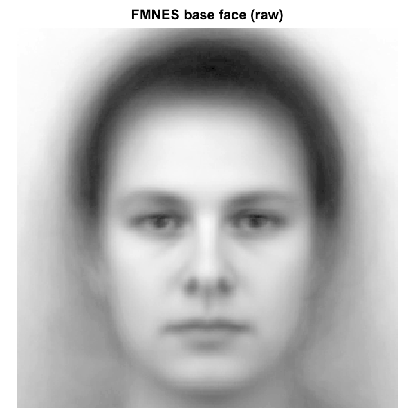
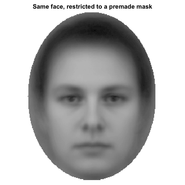
Effect of a face-region mask on a base image. Left: raw base face from the Karolinska Directed Emotional Faces database (KDEF; Lundqvist, Flykt, & Öhman, 1998). Right: same face with a premade full-face oval mask applied; pixels outside the mask are dimmed to light gray to make the analyzed region explicit. The reliability and discriminability metrics in this package will only see the inside-mask pixels when a mask is supplied via the mask argument.

When make_face_mask() is used to generate the mask parametrically, eight region presets are available. Imposed on the same base face (an artificial face generated with thispersondoesnotexist.com so no consent or licensing concerns apply), they look as follows. Five regions are ellipses (full, nose, mouth, upper_face, lower_face); the three eye regions (eyes, left_eye, right_eye) are axis-aligned rectangles, tunable to a specific base via the region_bounds argument (see the tuning subsection below). All eight region geometries are this package’s heuristics for a centered-portrait base; they are not taken from any specific published paper. The convention of applying a full-face oval before pixel-wise metrics follows prior practice in social-face RC (e.g., Oliveira et al., 2019; Ratner et al., 2014; Schmitz, Rougier, & Yzerbyt, 2024).

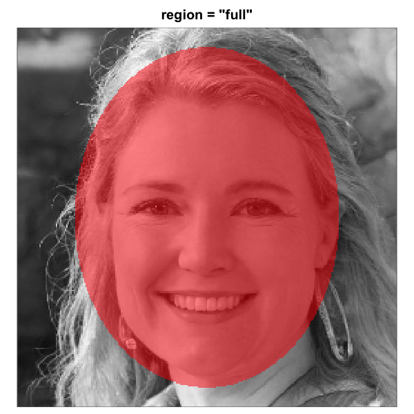
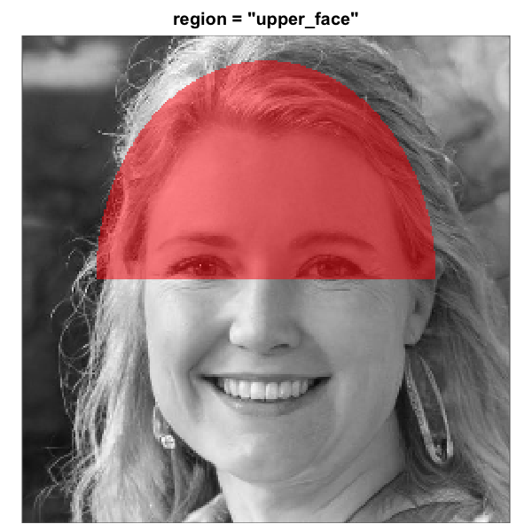
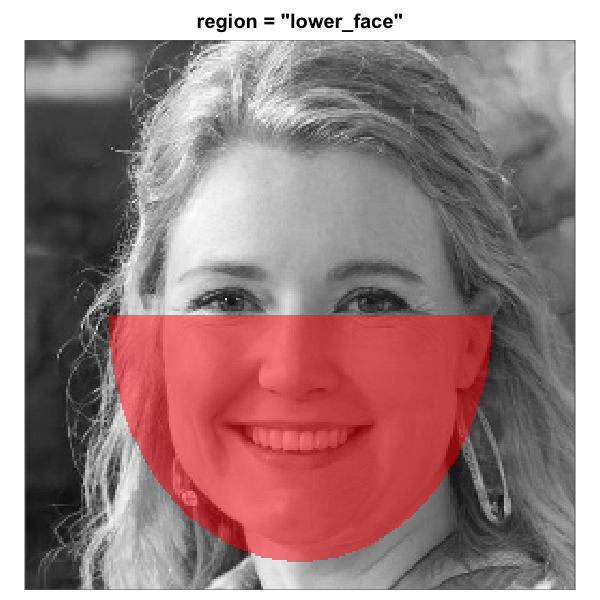
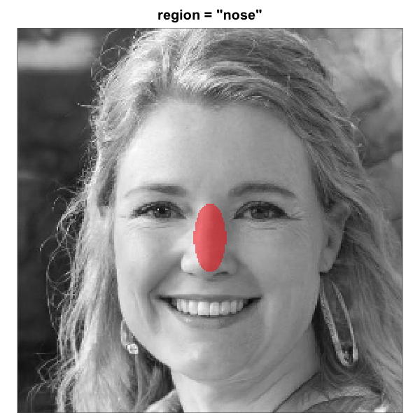
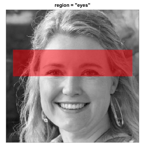
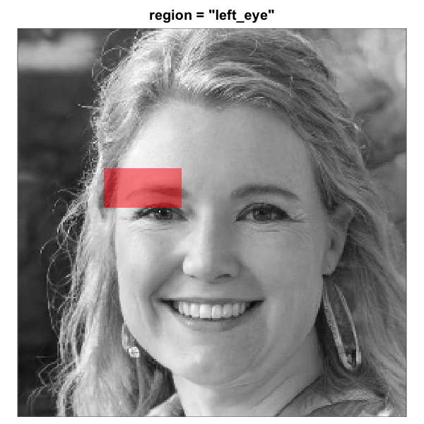
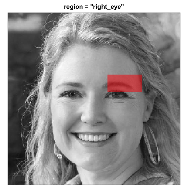
The eight built-in face-region masks rendered over the same artificial-person base face (256 x 256). Each translucent red overlay marks the pixels that pass through the mask; pixels outside are excluded from the analysis. All eight region geometries are this package’s heuristics for a centered-portrait base. The three rectangle eye regions are independent of the full-oval geometry and tunable via region_bounds.

The default geometry assumes the eyes sit roughly in the upper third of the image and the mouth in the lower third (centered square base, face filling most of the frame). Pass centre, half_width, and half_height to make_face_mask() if your base image has different framing.

Tuning a sub-region for a non-default base face

The default sub-region geometry is calibrated for a centered, frontal base face that fills most of the frame. The elliptical regions are positioned relative to the full-face oval (centre, half_width, half_height); the rectangle eye regions are independent of the oval and tuned via their own region_bounds. When the base image violates the centered-portrait assumption, the parametric overlay drifts off the intended feature and the metrics computed against it no longer mean what their name implies.

There are two tuning routes, depending on the region’s shape:

• Rectangle regions ("eyes", "left_eye", "right_eye") take a region_bounds = c(row_min, row_max, col_min, col_max) argument that sets the rectangle’s edges directly in 0-1 image fractions. Independent of the full-oval geometry; the rectangle for either eye can move without dragging the other along.
• Elliptical regions ("full", "nose", "mouth", "upper_face", "lower_face") are positioned relative to the full-face oval and tuned via the global centre, half_width, half_height. For independent per-region adjustment of an ellipse (a common need with non-portrait or AI-generated bases), the exported shift_mask() helper slides the mask by a number of pixels in any direction.

Rectangle regions: tune region_bounds

region_bounds accepts a length-4 numeric vector c(row_min, row_max, col_min, col_max) in 0-1 image fractions. Each pair must satisfy row_min < row_max and col_min < col_max, and every entry must lie in [0, 1]. The left and right eye rectangles are independent, so each can be nudged separately to match a specific base.

# Tune just the viewer's left-eye rectangle on a base whose
# eye line sits a few percent below the heuristic default. The
# right-eye rectangle is unaffected.
left_eye_tuned <- make_face_mask(
  c(256L, 256L), region = "left_eye",
  region_bounds = c(0.40, 0.50, 0.24, 0.44)
)

# Verify the alignment visually before passing to a metric.
# plot_mask_overlay() also accepts a `region =` shortcut that
# builds the mask internally; pass region_bounds the same way.
plot_mask_overlay(base_image = "data/base.png",
                  region = "left_eye",
                  region_bounds = c(0.40, 0.50, 0.24, 0.44))

If you measured the rectangle’s edges in pixels (by zooming into the base image in your viewer or plot() window), use region_bounds_from_pixels() to convert to the 0-1 fractions region_bounds expects:

# "The viewer's left eye sits in rows 100-130, cols 60-115 on
# this 256-pixel base." Convert once, pass straight through.
bounds <- region_bounds_from_pixels(
  row_min = 100, row_max = 130,
  col_min = 60,  col_max = 115,
  img_dims = c(256L, 256L)
)
make_face_mask(c(256L, 256L), region = "left_eye",
               region_bounds = bounds)

Rendered over the artificial-person base used earlier, the default left_eye rectangle and the tuned variant look as follows:

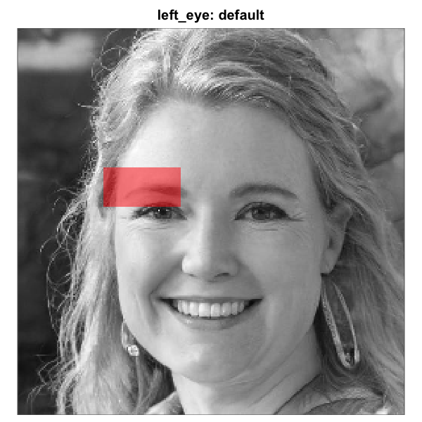
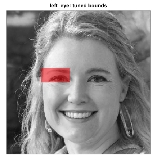
Rectangle left_eye mask before and after tuning on a base face whose eye line sits below the default. Left: default region_bounds, sitting on the eyebrow. Right: nudged downward by passing region_bounds = c(0.40, 0.50, 0.24, 0.44). Because the rectangle eye regions are independent of the full-oval geometry, the right-eye rectangle would remain untouched.

Elliptical regions: global centre or per-region shift

If every feature is offset in the same direction, pass the global centre (and optionally half_width, half_height) to make_face_mask():

# Whole-face shift: nose, mouth, and the full oval all move
# together. Rectangle eye regions are unaffected.
make_face_mask(c(256L, 256L), region = "mouth",
               centre = c(0.55, 0.50))   # 5% down

For independent per-region tuning of an ellipse, the exported shift_mask() helper slides the mask by a number of pixels in any direction. Pixels shifted off the image are dropped, and the newly exposed edge is filled with FALSE.

# Default mouth mask, reshaped from a flat logical vector
# (pixels in column-by-column order) back into a 256 x 256
# grid.
mouth_mask_default <- matrix(
  make_face_mask(c(256L, 256L), region = "mouth"),
  nrow = 256, ncol = 256
)

# Tune. Sign convention follows the math / y-axis-up idiom:
# positive `vertical` moves the mask up, negative moves it down;
# positive `horizontal` moves it right, negative moves it left.
# On this base the actual mouth sits *above* the default mask,
# so we shift up. 20 pixels is about 8 % of the 256-pixel
# height; 8 pixels is about 3 % of the width.
mouth_mask_v  <- shift_mask(mouth_mask_default, vertical = 20)
mouth_mask_vh <- shift_mask(mouth_mask_default,
                            vertical = 20, horizontal = 8)

shift_mask() accepts both vertical and horizontal offsets and combines them in a single call, so vertical-only and vertical-plus-horizontal tuning share the same idiom. It works on either a column-major logical vector (pass img_dims) or a logical matrix (returned in the same shape). Both infoval() and the rel_*() family accept a logical matrix as the mask argument, so the tuned grid can be passed in directly without flattening.

Rendered over the same artif_base.png shown earlier (where the mouth sits above the default), the default mask and the two tuned variants look as follows:

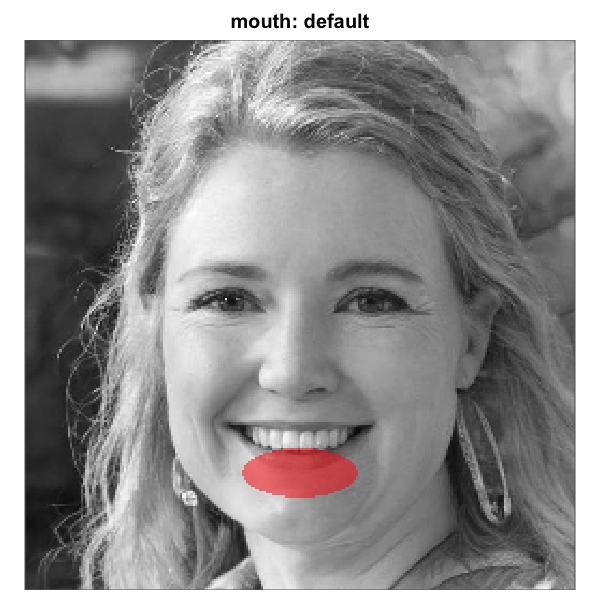
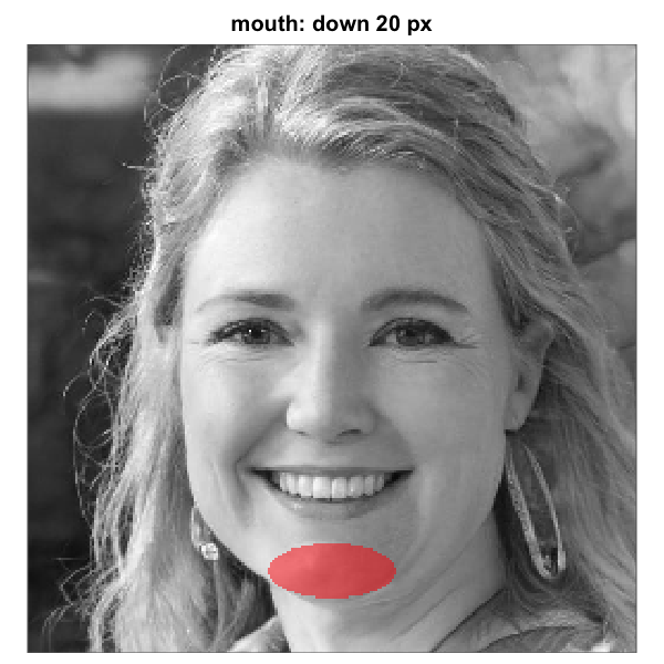
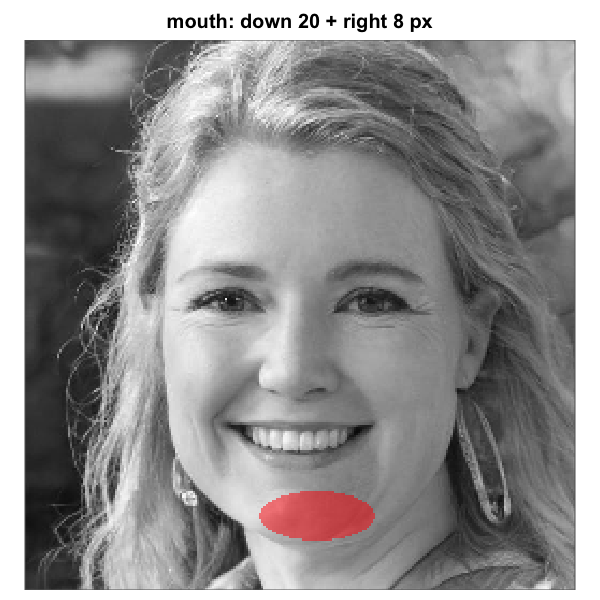
Elliptical mouth-region mask before and after shift-tuning on a base face whose mouth sits above the default. Left: default geometry. Middle: shifted up by 20 pixels (vertical = 20; about 8 percent of image height). Right: same vertical shift plus an 8-pixel rightward shift (vertical = 20, horizontal = 8). Each panel renders one of the matrices produced by shift_mask() above. The sign convention follows the math / y-axis-up idiom: positive vertical moves the mask up, negative moves it down; positive horizontal moves it right, negative moves it left. The same recipe works for nose, upper_face, lower_face, and the full oval; the three rectangle eye regions use region_bounds instead.

Iterate with plot_mask_overlay() (overlay on the base image) or plot_face_mask() until the overlay sits where you want, then pass the tuned mask to infoval() or any rel_*() function exactly as you would a parametric mask. Useful shift magnitudes are typically a few pixels to a few dozen on a 256-pixel image; if you find yourself needing more than that, the whole face is probably misaligned and centre should be retuned at the global level via make_face_mask() instead.

5. Diagnose the inputs

Before computing CIs, run the diagnostic battery. Two top-level entry points cover this step. run_diagnostics() (§5.1) invokes every implemented check whose required inputs are available and gathers the results into one printable report. infoval_report() (§5.4) is the focused per-producer infoVal report for the single question “is my data informative at all?”; it is the function to reach for when the headline worry is signal strength rather than coding or balance.

5.1 A first run

The smallest meaningful call needs only the response data and the method:

report <- run_diagnostics(responses, method = "2ifc")
report

The output looks like:

== Data-quality report (2ifc) ==

[PASS] Response coding
  All 60,000 responses coded {-1, 1}.
[PASS] Trial counts
  All 200 producers at 300 trials.
[PASS] Duplicates
  No duplicate rows.
[PASS] Response bias
  No constant responders, no |mean| > 0.6.

Summary: pass=4, warn=0, fail=0, skip=0

Skipped checks:
  - check_rt (no col_rt)
  - check_stimulus_alignment (no rdata or noise_matrix)
  - check_version_compat (no rdata)
  - infoval_report (no rdata + infoval_iter)
  - check_response_inversion (no rdata + infoval_iter)
  - check_rt_infoval_consistency (no rdata + infoval_iter + col_rt)

The “Skipped checks” block is informational, not a failure: each listed check has prerequisites the call did not supply. The next section walks through how to unlock each.

5.2 The result object

run_diagnostics() returns an rcisignal_diag_report with three fields:

• $results: a named list of rcisignal_diag_result objects, one per check that ran.
• $skipped_checks: character vector naming checks that were not run, each with the reason in parentheses.
• $method: "2ifc" or "briefrc".

Each rcisignal_diag_result has:

• $status: one of "pass", "warn", "fail", or "skip".
• $label: short check name.
• $detail: character vector of explanation lines.
• $data: optional list of programmatic data (flagged participants, count tables, group-level statistics).

summary(report) returns a flat data frame with check, status, label columns for programmatic filtering. print() is the human-readable view shown above.

5.3 The check_* family

Eight individual check functions cover the input-side battery. Each takes responses plus its check-specific arguments and returns an rcisignal_diag_result.

• check_response_coding() verifies {-1, +1} coding. PASS for {-1, 1}; WARN with a recode formula for {0, 1} or {1, 2}; FAIL otherwise. The {0, 1} miscoding produced by experiment software that records “left” / “right” as 0 / 1 is a common silent failure in 2IFC.
• check_trial_counts(expected_n = ...) verifies that every producer has the expected number of trials. expected_n can be a scalar or a named vector. PASS if all match; WARN at <= 10% off; FAIL above.
• check_duplicates() flags duplicate rows. PASS at 0; FAIL if >= 2 full duplicates and > 5% of rows; WARN otherwise.
• check_response_bias(bias_threshold = 0.6) flags constant responders (FAIL) and producers with |mean(response)| > bias_threshold (WARN; default 0.6 corresponds to roughly an 80/20 split).
• check_rt(col_rt = ...) scans response times for fast-clicking (default RT < 200 ms), implausibly slow trials, and low within-subject coefficient of variation. Defaults are conservative; tune them to your task.
• check_stimulus_alignment(rdata = ... | noise_matrix = ...) validates that stimulus ids fall inside the pool. FAIL on any out-of-range id; WARN if > 50% of the pool is unreferenced.
• check_version_compat(rdata = ...) (2IFC only) compares the generator_version recorded in the rdata to the installed rcicr version. PASS if matching; WARN otherwise. The warning is informational (older datasets remain usable, and the flag simply prompts a spot-check).
• check_response_inversion(rdata = ... (2IFC) | noise_matrix = ... (Brief-RC), infoval_iter = ...) detects whole-batch sign-flipped data by computing per-producer infoVal with the original responses and again with the negated responses. FAIL if >= 50% of producers are flagged as inverted; WARN if any are.

5.4 infoval_report()

infoval_report() is the canonical per-producer infoVal summary for the question “is my data informative at all?”. It runs six steps that surface the per-producer z-scores plus the calibration cross-checks that show whether those numbers can be trusted:

1. Compute observed Frobenius norm per producer (and group-mean).
2. Compare against a reference distribution at each producer’s actual trial count (closes the calibration gap in rcicr::generateReferenceDistribution2IFC(), which keys on pool size).
3. Apply a face mask (default "auto" = parametric full-face oval) and repeat.
4. Compare unmasked vs masked z to see whether masking lifts or depresses signal.
5. Sanity-check with a synthetic random responder (should land near 0; |z| > 2 flags a mis-calibrated reference).
6. Report whether the group-mean CI clears z = 1.96 even when per-producer medians do not.

iv <- infoval_report(
  responses,
  method    = "2ifc",
  rdata     = "rcic_stimuli.Rdata",
  iter      = 1000L,
  face_mask = "auto",
  seed      = 1L
)

iv  # PASS / WARN / FAIL with rich data attached to $data

The status logic:

• PASS: group-mean masked z >= 1.96 and random-responder z is within |z| < 1. Data is healthy.
• FAIL: random-responder |z| > 2. Reference distribution is miscalibrated; almost always indicates a noise-matrix or pool-id mismatch.
• WARN: anything in between. Usually means the per-producer signal is genuinely modest but the group CI is informative.

5.5 check_rt_infoval_consistency()

Cross-validates infoVal against RT quality by correlating per-producer infoVal with per-producer median RT. A strong negative correlation (correlation <= -0.30) suggests that fast clickers are also producing low-infoVal masks, indicating a population-level pattern rather than a single-producer fluke. WARN if the correlation passes the threshold; PASS otherwise. Works with both 2IFC (rdata = ...) and Brief-RC (noise_matrix = ...) data.

5.6 Conditional checks and required arguments

When the call carries only response data, four checks run and six are skipped. Each skipped check requires a specific additional argument:

Check	Required argument
check_rt	col_rt
check_stimulus_alignment	rdata (2IFC) or noise_matrix (Brief-RC)
check_version_compat	rdata (2IFC only)
infoval_report	rdata (2IFC) or noise_matrix (Brief-RC) + infoval_iter
check_response_inversion	rdata (2IFC) or noise_matrix (Brief-RC) + infoval_iter
check_rt_infoval_consistency	rdata (2IFC) or noise_matrix (Brief-RC) + infoval_iter + col_rt

infoval_iter defaults to NULL because the reference distribution simulation at 10,000 iterations takes minutes on first call. Opt in explicitly when you are ready to wait.

report <- run_diagnostics(
  responses,
  method       = "2ifc",
  rdata        = "rcic_stimuli.Rdata",
  base_image    = "base",
  col_rt       = "rt",
  expected_n   = 300L,
  infoval_iter = 1000L,
  face_mask    = "auto"
)

With every input supplied, the “Skipped checks” block is empty.

6. Compute classification images

Once the diagnostics pass, compute CIs.

6.1 From raw responses

The 2IFC path delegates to rcicr::batchGenerateCI2IFC() and returns a list with $signal_matrix (raw mask, ready for rel_*), optionally $rendered_ci for visualization, plus metadata.

# `responses` is a data frame loaded from CSV (see section 4.1).
res <- ci_from_responses_2ifc(
  responses,
  rdata_path    = "rcic_stimuli.Rdata",
  base_image    = "base",   # label from rdata, a path, or a numeric matrix
  scaling       = "none",   # raw mask only; render later if needed
  keep_rendered = FALSE
)

dim(res$signal_matrix)   # n_pixels x n_participants

Behind the scenes the function takes care of the steps that are easy to get wrong when calling rcicr directly: it loads the helper packages rcicr expects (foreach, tibble, dplyr) and checks that responses are coded {-1, +1}.

The two CI builders accept base_image the same way: a numeric matrix in [0, 1], a path to a PNG / JPEG, or (for 2IFC) a label naming an entry in the rdata’s base_faces list. Pass whichever form you already have.

The Brief-RC implementation follows Schmitz’s genMask() formula step for step, including the rule that collapses repeated stimulus ids by averaging their responses:

res <- ci_from_responses_briefrc(
  responses,
  rdata_path = "rcic_stimuli.Rdata",  # for the noise pool
  base_image = "base.jpg",            # path or numeric matrix in [0, 1]
  method     = "briefrc12"
)

You can pass a pre-loaded noise_matrix instead of rdata_path; useful when you have a non-rcicr-generated pool (e.g. Schmitz’s OSF text matrix).

Both builders return one column per producer in $signal_matrix. To average across producers into a single group CI (or several side-by-side group CIs for between-condition comparisons), pass group_by = to the builder, or call group_ci() directly. See section 1.3.

6.2 From pre-rendered CIs

When you already have one CI image per producer on disk (PNG or JPEG), read_signal_matrix() reads them and subtracts the base image in one call:

signal <- read_signal_matrix(
  dir             = "data/cis_condition_A/",
  base_image_path = "data/base.jpg"
)
dim(signal)   # n_pixels x n_producers

read_cis() and extract_signal() are also available on their own, for cases where you want to do something between reading the PNGs and subtracting the base (e.g. masking, cropping, or swapping the base image).

The first call to any Mode-1 reader emits the once-per-session warning that PNG-derived signals are scaled. Silence with options(rcisignal.silence_scaling_warning = TRUE) or pass acknowledge_scaling = TRUE when calling.

6.3 CI scaling options

rcicr::batchGenerateCI2IFC() exposes a scaling argument with five values:

• "autoscale": stretches each producer’s mask to a fixed symmetric range. The rcicr default and the convention used in Schmitz et al.
  2024. Experiment 2.
• "matched": stretches each mask to the base image’s range. Per-CI, so it breaks correlation-based metrics as well (a uniform scaling preserves Pearson, but a per-CI stretch does not).
• "independent": like autoscale with each CI’s stretch computed independently (no shared range across CIs).
• "constant": multiplies the mask by a fixed constant.
• "none": no scaling. Output is base + raw_mask.

Not every option is accepted by every builder: ci_from_responses_briefrc() takes "none", "matched", or "constant"; ci_from_responses_2ifc() takes "autoscale", "independent", "constant", or "none" (forwarded to rcicr).

The shipped $signal_matrix is the raw unscaled mask regardless of which scaling you pick; the scaling argument only affects the optional $rendered_ci field that keep_rendered = TRUE returns.

Recommendation: feed the raw $signal_matrix to every metric. For rcicr::computeInfoVal2IFC() the choice does not matter (it reads $ci internally). For Brief-RC, treat any non-none scaling as visualization-only and never pass it to rel_* or to hand-rolled infoVal.

7. Working with CIs: Typical workflow tour

With CIs computed in §6, this short hub answers four practical questions before the deeper metric chapters: which downstream section answers which analytical question, what is inside the result object, how do I pull one CI or a subset out for follow-up, and how do I view or mix CIs across the package’s visual surfaces. Every recipe here is a quick pointer; the metric chapters carry the depth.

7.1 Which section answers which question

Analytical question	Where in this guide
Are my CIs informative at all? (per-producer infoVal)	§10
Does the group-mean CI carry above-chance signal?	§11
Are producers in a condition consistent with each other? (within-condition reliability)	§8
Where do producers agree in pixel space, and where reliably?	§12.1, §12.2
Are two conditions distinguishable spatially? (cluster-based discriminability)	§9.2
How different in overall magnitude are two CIs, and is that above chance?	§9.3
How do several CIs order against each other? (correlogram / distance matrix / MDS)	§12.5-§12.7
How do I restrict any analysis to eyes / mouth / etc.?	§13
How do I get publication-ready PNGs of every CI to disk?	§1.4 (save_ci_images())

7.2 What’s inside the CI result object

ci_from_responses_briefrc() and ci_from_responses_2ifc() return a plain list. The fields downstream code consumes:

• $signal_matrix (pixels x producers, raw mask): the canonical input to every metric in §8-§12. Column names are the producer ids.
• $group_ci (pixels x groups): present when group_by = was supplied to the generator. Column names are the group labels (or underscore-joined factorial cell labels).
• $rendered_ci (pixels x producers, rescaled for display): never feed this to a metric (see §3.2 for the raw vs rendered distinction; the package aborts if a rendered matrix reaches a function that expects the raw mask).
• $participants, $img_dims, $scaling, $method are metadata.

res <- ci_from_responses_briefrc(
  responses,
  noise_matrix = noise,
  group_by     = "condition"     # also returns $group_ci
)

names(res)
str(res, max.level = 1)
colnames(res$signal_matrix)       # producer ids
colnames(res$group_ci)            # condition labels

For the deeper anatomy (raw vs rendered, the source / ci_level attributes, the three pixel matrices that all sound similar) see §3.

7.3 Pulling one CI or a subset out

Every column of $signal_matrix is one producer’s CI; every column of $group_ci is one group’s CI. Standard matrix subsetting pulls them out, with one detail: keep the result a matrix (drop = FALSE), because every downstream function expects a pixels-by-CIs matrix, not a bare vector.

# One individual CI.
one_ind   <- res$signal_matrix[, "P012", drop = FALSE]

# A chosen subset of individual CIs.
some_inds <- res$signal_matrix[, c("P012", "P015", "P019"),
                               drop = FALSE]

# One or more group CIs.
one_group  <- res$group_ci[, "happy", drop = FALSE]
two_groups <- res$group_ci[, c("happy", "sad"), drop = FALSE]

If you didn’t pass group_by = to the generator, build group CIs after the fact with group_ci():

grp <- group_ci(res$signal_matrix, responses, by = "condition")

by = accepts a single column name or a character vector for factorial groupings (c("condition", "sex"); cell labels joined with "_").

7.4 Viewing CIs

Two patterns cover almost every case:

# One CI on screen (individual or group).
plot_ci_overlay(res$signal_matrix[, "P012"],
                base_image = base, img_dims = res$img_dims)
plot_ci_overlay(res$group_ci[, "happy"],
                base_image = base, img_dims = res$img_dims)

# All CIs to disk, one PNG per column.
save_ci_images(res$signal_matrix, base_image = base, dir = "out/ind")
save_ci_images(res$group_ci,      base_image = base, dir = "out/group")

See §1.4 for save_ci_images() options (palette, JPEG output, custom prefix). See §12.3 for plot_ci_overlay() options (mask, contours from agreement_map_test(), alpha).

7.5 Mixing individual and group CIs in one comparison

plot_ci_correlogram(), plot_ci_distance_matrix(), and plot_ci_mds() each take a single matrix where every column is one CI. The columns can be any mix of individual producers and group averages. Build the matrix with cbind():

all_cis <- cbind(
  P012        = res$signal_matrix[, "P012"],
  res$group_ci      # all group columns
)
plot_ci_correlogram(all_cis,    img_dims = res$img_dims, mask = "face")
plot_ci_distance_matrix(all_cis, img_dims = res$img_dims, mask = "face",
                                method = "normalised")

Column names become the panel labels in the resulting figure; choose names that make the figure self-explanatory (e.g., P012_individual = res$signal_matrix[, "P012"], happy_group = res$group_ci[, "happy"]). See §12.5-§12.7 for the full options on each plot function.

8. Within-condition reliability

With the signal matrix in hand, the question is whether each condition’s group-level CI is stable: would you obtain the same group pattern from a different half of the producers? “Reliable” in the psychometric sense is shorthand for the producers’ CIs agree with each other enough that averaging them recovers the same pattern in repeated samples. Two complementary metrics address this question directly, alongside an influence-screening diagnostic that is sometimes confused with reliability.

The two reliability metrics:

• rel_split_half() asks how well one random half of the producers reproduces the other half’s group CI. Repeating the split many times gives a sampling distribution for the agreement.
• rel_icc() asks how much of the pixel-by-producer signal variance is attributable to consistent producer-level patterns versus residual noise. It is the same intraclass correlation used in measurement theory and inter-rater reliability work.

The third metric (rel_loo()) is an influence screen: it flags individual producers whose removal noticeably shifts the group CI, useful for catching coding errors or outlier strategies but not itself a reliability number.

A short note on what these metrics do not address. Reliability here is internal: would the same producers, if split differently, have produced the same CI? Whether the CI accurately captures the producer’s mental representation of the trait is a separate validity question, typically addressed by an external rater study, and sits outside the package.

8.1 rel_split_half()

Background. Split-half reliability is an old psychometric trick (Spearman, 1910; Brown, 1910): if a measurement is internally consistent, splitting it into two halves and correlating the halves should give a high correlation. In the RC setting, the “halves” are two random subsets of producers, and the quantities being correlated are the pixels of the group-mean CI computed from each half. The catch is that each half is built from N/2 producers rather than N, so the half-half correlation underestimates the reliability of the full N-producer CI. The Spearman-Brown correction r_sb = (2 r_hh) / (1 + r_hh) projects the half-half correlation up to the reliability the full sample would have if the underlying signal really is shared. Repeating the split many times and averaging both quantities reduces the dependence on any single random partition.

In code, the function does exactly this:

Randomly partition the producers into two halves, compute the group-level CI for each half (rowMeans()), correlate them, and average across many permutations. The function reports both the mean per-permutation r (r_hh) and the Spearman-Brown projected full-sample reliability (r_sb = (2 r_hh) / (1 + r_hh)). The headline number is typically r_sb.

sh <- rel_split_half(signal_matrix,
                     n_permutations = 2000L,
                     seed           = 1L)
sh
plot(sh)

Permutation is over producers (not pixels) so that each producer’s spatial structure is preserved. For odd N, one randomly-chosen producer is dropped per permutation (re-drawn each iteration) so both halves contain floor(N/2) producers.

The null argument adds an empirical chance baseline:

• null = "permutation": per iteration, generates fresh Gaussian noise per producer (no shared spatial structure), then recomputes r_hh. Centred at 0 and useful as a worst-case floor.
• null = "random_responders": simulates ncol(signal_matrix) random responders using the same genMask() machinery as infoval()’s reference. This baseline preserves the pixel correlation structure of real noise patterns and tracks the empirical chance baseline of an actual RC experiment more closely. Requires noise_matrix.

sh <- rel_split_half(signal_matrix,
                     null          = "random_responders",
                     noise_matrix  = nm,
                     n_permutations = 2000L,
                     seed          = 1L)

sh$r_hh                # observed
sh$r_hh_null_p95       # 95th percentile of the null
sh$r_hh_excess         # observed - null median
sh$r_sb_excess         # same, projected via Spearman-Brown

Report $r_sb as the headline; $r_sb_excess as the above-chance increment when a null is requested. $ci_95 / $ci_95_sb are percentile 95% CIs on the observed distribution.

8.2 rel_icc()

Background. The intraclass correlation coefficient (ICC) is a family of statistics for asking how much of the variability in repeated measurements is attributable to differences between the objects of measurement (here, producers) versus residual noise. The modern family of ICC variants was introduced by Shrout and Fleiss (1979), clarified and re-notated by McGraw and Wong (1996), and surveyed for practical reporting by Koo and Li (2016). Every producer has one CI vector with one entry per pixel, and the ICC asks how consistently the producers agree on that pixel-by-pixel pattern. A high ICC means producers’ CIs are similar to each other relative to noise; a low ICC means they are not.

The “(3,*)” label is the McGraw-Wong update of Shrout and Fleiss’s notation for a two-way mixed-effects model in which the column factor (pixels in our case) is fixed and the row factor (producers) is random. The fixed-pixels choice reflects the reality of an RC experiment: the image grid is not a random sample from a population of pixels; it is the same set of pixels across all producers. The “3,1 vs 3,k” distinction is whether you want the reliability of a single producer’s CI (3,1) or of the group-averaged CI across k producers (3,k).

rel_icc() returns both, computed from a two-way mixed model with pixels fixed and producers random:

• ICC(3,1) answers “how informative is one producer’s CI as a noisy estimate of the group pattern?”.
• ICC(3,k) answers “how stable is the group-mean CI across k producers?”. Usually the headline.

ic <- rel_icc(signal_matrix)
ic   # prints ICC(3,1), ICC(3,k), MS rows / cols / error

The function computes both quantities directly from ANOVA mean squares, which scales to large image grids that would otherwise run out of memory. Results agree with psych::ICC() on smaller matrices where both can be run.

ICC(3,) is appropriate when pixels are fixed. ICC(2,) (two-way random) treats pixels as a random sample from a pixel population, which the image grid is not, even when ICC(2,) and ICC(3,) give similar numbers at high pixel counts. Use variants = c("3_1", "3_k", "2_1", "2_k") to report ICC(2,*) side-by-side when comparability with reports that use the two-way-random model is needed.

ICC is variance-based, so it errors on a "rendered" source matrix unless acknowledge_scaling = TRUE is passed. Rendered scaling corrupts ICC values in non-recoverable ways, so the default behavior is conservative.

ICC(3,k) is the reliability of the group-mean CI across the k producers, so like any average-measures ICC it rises with the number of producers (Spearman-Brown: ICC(3,k) = k * ICC(3,1) / (1 + (k - 1) * ICC(3,1)), which approaches 1 as k grows). It is therefore not comparable across studies that pooled different numbers of producers; report ICC(3,1), the single-producer reliability, for cross-sample comparisons.

Both ICCs also depend on which pixels enter the computation. When the signal is localized to a few face regions, an unmasked full-image ICC is diluted by the many off-signal background pixels and can be driven toward zero, more so at higher resolutions. Restrict the computation to the analysis region with mask = make_face_mask(...) for an interpretable value. A once-per-session warning fires when ICC(3,k) is requested over more than 50,000 pixels, as a reminder of both points.

Empirically, ICC(3,k) and the group-mean infoVal z (see §10) track each other very closely on real data: both quantify how aligned the producers are on the pixel-level signal, ICC(3,k) as a variance ratio and group-mean z as the magnitude of the surviving group-mean signal against a matched reference. §14.6 shows the empirical relationship across ten trait conditions on the Oliveira et al. (2019) data (Pearson r ≈ 0.97).

8.3 rel_loo()

Background. Leave-one-out (LOO) is a jackknife-style influence diagnostic (Tukey, 1958; Cook, 1977): for each producer in turn, recompute the group CI with that producer removed and correlate the result with the full-sample group CI. Producers whose removal changes the group CI more than the others stand out as high-influence cases worth a closer look. This is not a reliability metric. The with-producer and without-producer group CIs share (N-1)/N of their data, so LOO correlations are near 1 by construction even on noisy data; the diagnostic information lives in the relative ordering of producers, which the function summarizes as a robust z-score.

For each producer i, this function computes the Pearson correlation between the full-sample group CI and the group CI recomputed without producer i. Producers whose r_loo sits well below the others are candidates for inspection.

lo <- rel_loo(signal_matrix)
lo                       # raw cors + z-scores + flag column
rel_loo_z(lo)            # tidy data frame, sorted by z_score
plot(lo)

r_loo values typically sit in the [0.95, 0.999] range at N = 30 (near 1 by construction, per the Background note above), so the function reports $z_scores as the headline diagnostic.

Two flagging rules are available: "mad" (default) and "sd". MAD is robust to the influential producers the test is meant to flag; SD’s mean and standard deviation are themselves pulled by the outlier. Default flag_threshold = 2.5 so that a 30-producer dataset flags ~0.3 producers by chance.

A flag prompts inspection rather than exclusion. Investigate first (response coding, fatigue, atypical strategy) and cross-check with run_diagnostics() to rule out coding errors before excluding any producer.

8.4 run_reliability()

Top-level convenience function that runs rel_split_half() and rel_icc() on a single signal matrix and bundles both results into one rcisignal_rel_report:

rep <- run_reliability(signal_matrix,
                       n_permutations = 2000L,
                       seed           = 1L)
rep
plot(rep)

rep$results$split_half and rep$results$icc are the standalone result objects. run_reliability() deliberately omits rel_loo(), since LOO is an influence-screening diagnostic and bundling it into a reliability report invites misreading r_loo’s near-1 values as reliability.

9. Between-condition discriminability

When the design has two or more conditions, the question becomes whether their group CIs are distinguishable, both in overall magnitude and in spatial location.

The hard part of doing this honestly is the multiple comparisons problem. A typical RC image has tens of thousands of pixels (a 256 x 256 grid has 65,536). If you compute one t-test per pixel and threshold each at the conventional p < 0.05, you should expect about 5% of pixels to come out “significant” by chance even when the two conditions are identical, which is over 3,000 false-positive pixels per image. The naive Bonferroni correction (divide alpha by the number of tests) overcorrects in the opposite direction because pixels are spatially correlated; CI signal lives in contiguous regions, not independent dots.

The solution adopted here is borrowed from the neuroimaging literature: build a single test statistic that summarizes the spatial extent of the effect (a cluster), and calibrate it against a null distribution generated by random label permutation. This controls the family-wise error rate (FWER) in the strong sense, that is, the probability of one or more false positives anywhere in the image is held below the chosen alpha (Nichols & Holmes, 2002; Maris & Oostenveld, 2007). Two test statistics are offered:

• A classical cluster-mass statistic with a user-set cluster- forming threshold (rel_cluster_test(method = "threshold")).
• Threshold-free cluster enhancement, TFCE (rel_cluster_test(method = "tfce"); Smith & Nichols, 2009), which sidesteps the threshold choice by integrating the cluster contribution to each pixel across many thresholds.

A complementary question is the overall magnitude of the difference, independent of where in the image it sits. rel_dissimilarity() addresses that with a single distance number plus a bootstrap confidence interval.

Which pairings work. pixel_t_test(), rel_cluster_test(), and rel_dissimilarity() all take two signal matrices A and B and ask “how do they differ?”. The two arguments can be:

• group vs group: each matrix has many producer columns, one group per matrix. The canonical case (compare condition A to condition B). All three functions and their bootstrap / permutation nulls are designed for this pairing.
• individual vs individual: each matrix is a single-column CI for one producer (use [, "P012", drop = FALSE]). The point estimate (t-map for pixel_t_test(), distance for rel_dissimilarity()) is interpretable, but the inferential statistics degenerate: bootstrap CIs collapse for n = 1, the per-pixel Welch t has zero residual degrees of freedom, and cluster permutation produces a trivial null. Treat these as descriptive comparisons only; for an inferential comparison between two individual CIs you need at least a few producers on each side.
• individual vs group, or two individuals from the same condition: same call shape, same descriptive-only caveat. Useful for asking “how far is this one producer from the group mean of another condition?”.
• all-vs-all descriptive distance for a set that mixes individuals and groups: build a single matrix with cbind() (see §7.5) and hand it to plot_ci_distance_matrix() or plot_ci_correlogram(). These do not run inferential statistics; they report the descriptive distance / correlation between every pair.

9.1 pixel_t_test()

Background. The pixel-wise t-test is the building block of everything in this section: at each pixel, compare the two conditions’ producer-level signal values with a Welch’s t (or a paired t when producers are matched). The output is one t-value per pixel, an image-shaped statistical map of where the conditions differ.

This map is informative, but it is not a valid statistical test on its own. With tens of thousands of pixels and no multiplicity correction, raw per-pixel p-values overstate the strength of evidence (see the §9 intro above). For that reason pixel_t_test() returns the t-vector and stops there; turning it into inference is the job of rel_cluster_test() (§9.2), which feeds these per-pixel t-values into a permutation-based FWER procedure.

In code:

Vectorised Welch’s t (independent groups) or paired t (matched producers) per pixel:

t_vec <- pixel_t_test(signal_a, signal_b)         # n_pixels long
t_vec_paired <- pixel_t_test(signal_a, signal_b,
                             paired = TRUE)

Returns a numeric vector of t-values, length n_pixels (or sum(mask) if a mask is supplied). The function serves as an intermediate building block for rel_cluster_test() and is not intended as a standalone inferential test (no FWER control at the per-pixel level). For paired mode, the two matrices must have identical ncol and matching column names.

9.2 rel_cluster_test()

Background. The cluster-based permutation test (Maris & Oostenveld, 2007) treats the spatial coherence of CI signal as a feature, not a nuisance. The procedure is in three conceptual steps:

1. Compute the per-pixel t-statistic (as in §9.1), and threshold its absolute value at some cutoff (e.g., |t| > 2). Each pixel is either supra-threshold or not.
2. Group the supra-threshold pixels into spatially contiguous clusters using a neighbor rule. The default in rcisignal is 4-connectivity: a pixel’s neighbors are the four pixels sharing an edge with it (up, down, left, right). 8-connectivity (which also counts diagonal neighbors) tends to merge things that only touch at a corner, producing larger and fewer clusters; 4-connectivity is the conservative default and is the one used here.
3. Score each cluster by its mass: the sum of the t-values inside the cluster. A small cluster of very high t-values can have the same mass as a large cluster of moderate t-values, and the mass statistic treats them as comparably strong evidence.

The hard part is calibration: how big a cluster mass would you expect under the null (the conditions are identical)? The permutation answer is to randomly relabel which producer is in which condition (preserving the per-condition N), recompute the per-pixel t and the maximum cluster mass, and repeat thousands of times. The resulting distribution of maximum cluster masses is the empirical null, calibrated to your data without distributional assumptions. A real cluster’s p-value is the fraction of null max-masses that exceed it. Because every candidate cluster is tested against the maximum cluster mass under the null, the family-wise error rate is controlled for the family of clusters — the probability of finding one or more false-positive clusters under H0 is bounded by alpha. This is the form of FWER control proposed by Maris and Oostenveld (2007); the precise pixel-level extent of a significant cluster is only weakly controlled (Maris & Oostenveld, 2007, §4.4.3), so cluster boundaries should be read as “the broad region survives the family-wise correction” rather than “every pixel inside the contour is individually FWE-significant”. For pixel-level strong FWER control the relevant test is the voxel-wise max-statistic permutation used in §12.1’s agreement_map_test() (Nichols & Holmes, 2002).

One caveat: the cluster-forming threshold does not have a fully principled default. Lower thresholds favor broad and diffuse effects; higher thresholds favor focal and intense ones (Smith & Nichols, 2009). When you do not have prior intuition about the spatial scale of your effect, TFCE (below) avoids having to choose.

In code, rel_cluster_test() exposes both methods.

method = "threshold" (default; Maris & Oostenveld 2007): threshold |t| > cluster_threshold (default 2.0), label connected components with 4-connectivity (the conservative choice over 8-connectivity), and use cluster mass (sum of t-values within the cluster, not pixel count) as the test statistic. The null is built by stratified label permutation: every permutation preserves (N_a, N_b) exactly, the pixel-wise t is recomputed on shuffled labels, and the maximum positive and maximum negative cluster masses are recorded. A cluster’s p-value is the fraction of null masses (matching sign) that exceed the observed.

ct <- rel_cluster_test(
  signal_a, signal_b,
  img_dims          = c(256L, 256L),
  cluster_threshold = 2.0,
  n_permutations    = 2000L,
  alpha             = 0.05,
  seed              = 1L
)
ct
plot(ct)

The result carries $clusters (a data frame with cluster_id, direction, mass, size, p_value, significant), $null_distribution (the $pos and $neg per-permutation max masses), and integer label matrices $pos_labels / $neg_labels for plotting. Maximum-cluster-mass permutation provides FWER control at the cluster-family level (the probability of any false-positive cluster under H0 is bounded by alpha); pixel-level localization within a significant cluster is only weakly controlled (Maris & Oostenveld, 2007).

method = "tfce" (Smith & Nichols 2009): threshold-free cluster enhancement. Instead of picking one cluster-forming threshold, TFCE walks across many possible thresholds and adds up, at each pixel, how much spatial support the surrounding cluster has at each threshold height. Pixels embedded in strongly-supported clusters end up with high TFCE scores; isolated pixels with no neighbor support end up with low scores. Per-pixel TFCE value is the integral over thresholds of size^E x h^H x dh; positive and negative tails are enhanced separately and recombined with sign preserved. No free threshold parameter to choose. Per-pixel p-value = (sum(null_max_abs_tfce >= |observed_tfce|) + 1) / (n_perm + 1).

ct_tfce <- rel_cluster_test(
  signal_a, signal_b,
  img_dims = c(256L, 256L),
  method   = "tfce",
  tfce_H   = 2.0,
  tfce_E   = 0.5,
  seed     = 1L
)

Defaults match Smith & Nichols (H = 2.0, E = 0.5, n_steps = 100). TFCE result carries $tfce_map, $tfce_pmap, $tfce_significant_mask instead of $clusters. Print and plot methods branch on $method.

For a paired design, pass paired = TRUE; the per-pixel statistic becomes paired t and the null is built by random sign-flip on per-producer differences (exact under exchangeability of pair sign).

9.3 rel_dissimilarity()

Background. The Euclidean distance between two CIs is the square root of the summed squared pixel differences (equivalently, the Frobenius norm of the difference matrix). Writing $\bar{A}_i$ and $\bar{B}_i$ for the per-pixel group means at pixel $i$ across the producers in conditions A and B, and $\mathcal{M}$ for the set of in-mask pixel indices, the distance is

$$D(A, B) = \sqrt{\sum_{i \in \mathcal{M}} \left(\bar{A}_i - \bar{B}_i\right)^2}.$$

The optional normalised form

$$D_{\mathrm{norm}}(A, B) = \frac{D(A, B)}{\sqrt{\left| \mathcal{M} \right|}}$$

divides by the square root of the mask cardinality to make distances comparable across different image resolutions or different region masks (Brinkman et al., 2019, use the same Frobenius-norm reduction to single-number magnitudes for the related infoVal metric; see §10). This is the standard Euclidean distance on the flattened difference image. Other distance metrics exist (cosine, Mahalanobis, correlation distance) but rcisignal commits to Euclidean throughout, so that the single-pair number from rel_dissimilarity(), the all-vs-all matrix from plot_ci_distance_matrix(), and the MDS embedding from plot_ci_mds() are all on the same scale.

It is a single-number summary of how far apart two group CIs sit in pixel space. It ignores where the difference lives and reports only its overall magnitude. The advantage is simplicity: one number per contrast, comparable across studies, with a percentile bootstrap CI (resample producers with replacement, recompute the distance, repeat) for uncertainty. The trade-off is loss of spatial detail, which is exactly what rel_cluster_test() (§9.2) is for. Reported together, the two metrics complement each other: the cluster test localises the difference, the dissimilarity quantifies its overall size.

One caveat: Euclidean distance scales with image size and with whatever absolute units the CI carries. The $euclidean_normalised field divides by sqrt(n_pixels) to make distances comparable across resolutions, but cross-study comparison still requires care about scaling conventions and the underlying base image.

Why the bootstrap CI on the distance is not a test against zero. The Euclidean distance is a non-negative L2 norm. Resampling producers with replacement adds variance to each resampled group mean, and that variance enters the squared-distance sum at every pixel: $E\!\left[(\bar{A}^{*}_i - \bar{B}^{*}_i)^2\right] \approx (\bar{A}_i - \bar{B}_i)^2 + \mathrm{Var}(\bar{A}^{*}_i) + \mathrm{Var}(\bar{B}^{*}_i)$. Summed over thousands of pixels the upward bias is large, so the bootstrap distribution of the distance sits above the observed value and its CI almost always excludes zero, even when the two conditions come from the same population. The bootstrap CI therefore answers only “how stable is my distance estimate under producer resampling?”, not “is there a difference?”. To test the distance against chance, set null = "permutation": the null shuffles condition labels and recomputes the distance, so it is centred at the chance distance between two random subgroups of producers, which is positive, not zero. Reject only when the observed distance sits in the upper tail of that permutation null. The Pearson fields carry the mirror-image bias: resampling attenuates r, so its bootstrap CI sits below the observed value; benchmark r against a permutation null too.

In code, run the permutation null as the primary inferential output and keep the bootstrap CI as a secondary precision interval:

dr <- rel_dissimilarity(
  signal_a, signal_b,
  n_boot         = 2000L,
  null           = "permutation",
  n_permutations = 2000L,
  ci_level       = 0.95,
  seed           = 1L
)
dr

# Permutation p: proportion of null distances at or above the observed.
p_perm <- (1 + sum(dr$null_distribution >= dr$euclidean)) /
          (length(dr$null_distribution) + 1)

# Primary inferential summary.
c(d       = dr$euclidean,
  M_null  = mean(dr$null_distribution),
  SD_null = sd(dr$null_distribution),
  d_z     = dr$d_z,
  d_ratio = dr$d_ratio,
  p_perm  = p_perm)

plot(dr)

$euclidean is the observed distance and $euclidean_normalised is $euclidean / sqrt(n_pixels), useful for cross-resolution comparisons. The permutation summaries ($d_z, $d_ratio, $d_null_p95, and the permutation p above) are the inferential output: they place the observed distance against the positive-centred chance baseline. The bootstrap fields ($boot_dist, $ci_dist, $boot_se_dist) are a precision interval on the distance estimate, useful for judging how stable the number is under producer resampling and for comparing relative magnitudes across contrasts. They are not a test against zero, for the reason in the callout above.

The Pearson correlation fields ($correlation, $boot_cor, $ci_cor, $boot_se_cor) are returned as a secondary summary; they are not recommended as a standalone similarity score. Two base-subtracted CIs share image-domain spatial structure (face shape, oval signal support) that pushes their correlation above zero even when the underlying mental representations are unrelated, so a “high” absolute r can reflect shared image scaffolding rather than shared mental content. The bootstrap CI on r carries the opposite bias to the distance CI: producer resampling attenuates r, so the CI sits below the observed value rather than spanning it. Euclidean distance is the primary metric here.

If you do report r (for comparability with prior literature or with another analysis pipeline), interpret it relatively rather than absolutely: the ordering of r across multiple condition pairs is more defensible than any single value, and the right reference point is a permutation null (e.g., permute participant labels between conditions and recompute r) rather than zero. The image-domain scaffolding shifts the chance baseline upward, so “r > 0” is not the right test.

A worked illustration: identical conditions

When two conditions are drawn from the same population there is no real difference to detect, yet the bootstrap CI on the distance still excludes zero. The permutation null is what behaves correctly. The example below runs 60 such null datasets (two conditions of 20 producers each, drawn from the same distribution) and records, per dataset, whether the bootstrap CI excludes zero and the permutation p:

suppressPackageStartupMessages(library(rcisignal))
options(rcisignal.silence_scaling_warning = TRUE)
set.seed(7)
reps   <- 60L
n_pix  <- 24L * 24L   # small toy image, for speed
n_prod <- 20L

ci_excludes_zero <- logical(reps)
p_perm           <- numeric(reps)
first            <- NULL

for (r in seq_len(reps)) {
  # Two conditions from the SAME distribution: no real difference.
  A <- matrix(rnorm(n_pix * n_prod), n_pix, n_prod)
  B <- matrix(rnorm(n_pix * n_prod), n_pix, n_prod)
  d <- rel_dissimilarity(A, B, n_boot = 400L, null = "permutation",
                         n_permutations = 400L, progress = FALSE)
  ci_excludes_zero[r] <- d$ci_dist[1] > 0
  p_perm[r] <- (1 + sum(d$null_distribution >= d$euclidean)) /
               (length(d$null_distribution) + 1)
  if (r == 1L) first <- d
}

# One representative dataset: the bootstrap CI sits ABOVE the observed
# distance and well clear of zero, yet the permutation p is unremarkable.
c(observed_d = first$euclidean,
  ci_low     = first$ci_dist[1],
  ci_high    = first$ci_dist[2],
  p_perm_1   = (1 + sum(first$null_distribution >= first$euclidean)) /
               (length(first$null_distribution) + 1))
#> observed_d     ci_low    ci_high   p_perm_1 
#>  7.4024848  9.4964286 11.6554809  0.8354115

# Across all 60 null datasets.
c(pct_CI_excludes_zero = 100 * mean(ci_excludes_zero),
  mean_p_perm          = mean(p_perm),
  pct_p_perm_below_05  = 100 * mean(p_perm < 0.05))
#> pct_CI_excludes_zero          mean_p_perm  pct_p_perm_below_05 
#>          100.0000000            0.4707814           10.0000000

The bootstrap CI excludes zero in essentially every null dataset, which would license a “difference” claim that is simply wrong. The permutation p is centred near .5 (a single p is uniform under the null, so any one value is luck of the draw) and rejects at p < .05 only about as often as the nominal 5% rate. Read the distance against the permutation null, not against the bootstrap CI.

Choosing between Pearson r and Euclidean distance

rel_dissimilarity() returns both the Euclidean distance and the Pearson correlation between the two group-mean CIs. They answer different questions and have different baselines.

Pearson r is invariant to additive shifts and multiplicative rescaling of either CI. It asks “do these two CIs go up and down together across pixels?”. Euclidean distance is not invariant to either: it asks “how far apart are these two CIs in pixel space, in the same units as the underlying CI?”. For magnitude claims (does this contrast move pixels far apart in absolute terms?) distance is the answer; for pattern claims (do these two CIs vary in the same spatial way?) correlation is closer to the question, but with a baseline caveat described next.

Two base-subtracted CIs share image-domain spatial structure (face shape, oval signal support, scaling conventions of the underlying noise patches) that pushes their Pearson r above zero even when the underlying mental representations are unrelated. The right baseline for r between two CIs is therefore not zero but a permutation null built by shuffling condition labels (or sign-flipping differences in paired designs) and recomputing r. Euclidean distance is also not strictly baseline-free, but in practice the shared scaffolding contributes a roughly constant additive distance, so relative comparisons (“which two CIs are closest?”) survive without an explicit null. The worked example in §14.6 shows that the relative ordering of condition pairs by Pearson r matches the ordering by Euclidean distance on the Oliveira et al. (2019) data, but only the distance gives an interpretable absolute magnitude.

Practical recommendation: report Euclidean distance (raw, or normalised by $\sqrt{|\mathcal{M}|}$ when comparing across masks) as the primary single-number summary of how distinct two CIs are; use r as a secondary relative ordering inside a set of contrasts, and pair it with a permutation null if you need to make any “above-chance” claim about r itself.

9.4 run_discriminability()

Orchestrator that runs rel_cluster_test() and rel_dissimilarity() on a pair of signal matrices:

rep <- run_discriminability(signal_a, signal_b,
                            img_dims          = c(256L, 256L),
                            cluster_threshold = 2.0,
                            seed              = 1L)
rep
plot(rep)  # cluster t-map + bootstrap dissimilarity, side by side

plot(rep) is the one-call view of the whole report. The children rep$results$cluster_test and rep$results$dissimilarity are the standalone results, useful when you want a single panel with a custom title (for example to compare conditions named on a poster or a figure caption):

plot(rep$results$cluster_test,
     main = "US vs PT - cluster test")
plot(rep$results$dissimilarity,
     main = "US vs PT - bootstrap dissimilarity")

9.5 run_discriminability_pairwise()

Generalises run_discriminability() to all K-choose-2 pairs of K conditions, with a family-wise correction across pairs (Holm by default, Bonferroni or none also available):

rep <- run_discriminability_pairwise(
  signal_matrices = list(
    Trust    = sm_trust,
    Dominant = sm_dominant,
    Friendly = sm_friendly
  ),
  fwer = "holm",
  seed = 1L
)
rep$pairs   # one row per pair: cond_a, cond_b, p_min, p_adj_pair
plot(rep)   # cluster t-map per pair, laid out in a grid

plot(rep) lays out one cluster t-map per pair in a square-ish grid. A warning fires above max_pairs = 12 because at that density the panels become illegible; subset rep$results and plot a slice, or call plot(rep, max_pairs = Inf) to silence the warning. To inspect a single pair on its own, or to override the title:

plot(rep$results[["Trust_vs_Dominant"]]$cluster_test,
     main = "Trust vs Dominant")
plot(rep$results[["Trust_vs_Dominant"]]$dissimilarity,
     main = "Trust vs Dominant - bootstrap")

For a shared-axis comparison of bootstrap distances across pairs, pass each pair’s dissimilarity child to plot_dissimilarity_grid().

When the comparison is many conditions at once (rather than a short list of pairs), the all-vs-all summaries in §12.6 and §12.7 are the natural tools: plot_ci_distance_matrix() for a pairwise Euclidean-distance heatmap across N conditions, and plot_ci_mds() to project the same N CIs into a 2D / 3D / kD map with automatic Kruskal-stress-driven dimensionality selection.

The per-pair statistic carried into the across-pairs adjustment is the minimum cluster-level p-value within each pair; within-pair cluster p-values are not re-adjusted (they retain the max-statistic FWER control from the underlying rel_cluster_test()). A pair with no clusters contributes p_min = 1.0.

10. Per-producer informational value

Background. Per-producer infoVal (Brinkman et al., 2019) asks a single question: is this producer’s CI larger in magnitude than what a random responder would produce on the same task? The metric is a modified z-score. The numerator is the Frobenius norm of the CI mask (the square root of the summed squared pixel values, a scalar that summarizes overall mask “size”). The reference distribution comes from simulating many random (stimulus, ±1) response sequences through the same CI formula, computing the Frobenius norm of each simulated mask, and recording the median of those norms (the center) and the median absolute deviation (MAD) scaled by 1.4826 (the spread). Brinkman et al. use the modified z deliberately because the reference distribution of Frobenius norms is left-skewed; median and scaled MAD are robust substitutes for the mean and SD that would otherwise be distorted by the skew. A producer’s infoVal of, say, 2.5 means their CI is 2.5 scaled-MAD units above the random-responder median. The conventional threshold for “more than chance” is z >= 1.96, the standard normal cutoff Brinkman et al. adopt: a one-sided 2.5% (equivalently two-sided 5%) error rate.

What infoVal does not tell you is whether the CI points at the right pattern. The Frobenius norm is a magnitude statistic only. A producer who clicked consistently but in a way that encodes an unrelated visual pattern (for example, their CI looks like an upper-left versus lower-right contrast rather than a trait-relevant face feature) can still score high on infoVal. Pair infoVal with the reliability metrics (§8) and the discriminability metrics (§9) when you want a fuller picture.

Group-level signal summaries. For the group-mean z statistic (group_mean_z(), surfaced inside infoval_report()), the Brinkman-recommended primary group-level summary (the distribution of per-producer infoVals), and per-pixel agreement maps — including the reasoning behind the matched-N reference and a calibration illustration — see §11.

In code:

infoval() reports a per-producer Frobenius-norm z-score against a reference distribution matched to that producer’s actual trial count:

iv <- infoval(
  signal_matrix,
  noise_matrix,
  trial_counts,           # named integer vector matching colnames
  iter       = 10000L,
  mask       = make_face_mask(c(256L, 256L)),
  seed       = 1L,
  cache_path = "data/infoval_cache.rds"
)
iv$infoval         # named numeric: per-producer z-score
plot(iv)

What does infoval() iterate over?

infoval() returns one z-score per column of the signal matrix you hand it, against a reference distribution matched to that column’s trial count. The same call shape works regardless of whether the columns are individual producers, a chosen subset, or group CIs:

# (a) All producers at once. Standard per-producer infoVal.
infoval(res$signal_matrix, noise, trial_counts = tc)$infoval
#>     P001     P002     P003     ...
#>   1.834    0.412    2.611    ...

# (b) One specific producer. Pass a 1-column slice (drop = FALSE).
infoval(res$signal_matrix[, "P012", drop = FALSE], noise,
        trial_counts = tc["P012"])$infoval
#>     P012
#>   1.027

# (c) A chosen subset of producers.
keep <- c("P012", "P015", "P019")
infoval(res$signal_matrix[, keep, drop = FALSE], noise,
        trial_counts = tc[keep])$infoval

# (d) Group CIs. One z per group column, against a trial-count-
#     matched reference per group.
group_tc <- tapply(tc, responses$condition[match(names(tc),
                   responses$participant_id)], sum)
infoval(res$group_ci, noise,
        trial_counts = group_tc)$infoval
#>    happy      sad
#>   12.40    11.95

In each case infoval() just iterates over columns; the “per-producer vs per-group” distinction is entirely about what columns mean and what trial count their reference must match. For per-producer CIs trial_counts is the named vector of how many trials each producer contributed (which is what the responses table tells you via table(responses[[col_participant]]), or what the responses-aware form infoval(..., responses = responses, col_participant = "participant_id") derives for you). For group CIs the reference must be matched to the sum of the trial counts of the producers in that group, because the group CI is built from N producer masks summed (then averaged) at their individual trial counts. Passing a per-producer trial count for a group column would calibrate the reference against the wrong N and return a misleading z (see §17 for what goes wrong in detail; the per-producer / group-mean distinction there carries the same matching requirement).

The function unifies 2IFC and Brief-RC infoVal under one implementation. The only difference between paradigms is what you pass as noise_matrix. The reference distribution is built per unique trial count by simulating random (stim, ±1) pairs through Schmitz’s genMask() formula and computing Frobenius norms of the resulting masks. Producers sharing a trial count share a reference, so the simulation cost is paid once per distinct trial count rather than once per producer.

Trial-count matching closes a calibration gap. The original rcicr::generateReferenceDistribution2IFC() keys its reference on the full pool size. For 2IFC this is appropriate (every producer typically responds to every pool item). For Brief-RC, where the recorded number of mask contributions equals n_trials and is typically smaller than n_pool, a pool-size reference biases infoVal downward. infoval() uses each producer’s actual recorded trial count.

10.1 Validation against rcicr on real data

Because rcisignal::infoval() is a reimplementation, it is useful to know how its numbers line up with the established rcicr::computeInfoVal2IFC(). The companion vignette Validation: rcisignal vs rcicr infoVal convergence runs both implementations on the open data from Oliveira, Garcia-Marques, Dotsch & Garcia-Marques (2019), ten traits, twenty producers per trait, 300 trials each. The headline table:

trait	n	median z (rcisignal)	median z (rcicr)	n ≥ 1.96 (rcisignal)	n ≥ 1.96 (rcicr)	Pearson r
competent	20	0.089	0.083	2	2	1.000
dominant	20	0.268	0.267	4	4	1.000
friendly	20	0.703	0.713	1	1	1.000
incompetent	20	0.243	0.241	0	0	1.000
intelligent	20	0.584	0.591	2	2	1.000
submissive	20	0.525	0.530	4	4	1.000
trust	20	0.323	0.323	2	2	1.000
unfriendly	20	0.712	0.722	3	3	1.000
unintelligent	20	0.233	0.231	1	1	1.000
untrust	20	0.664	0.673	5	5	1.000

Two patterns stand out. First, the per-producer correlation is 1.000 in every trait, so the two implementations rank producers identically and produce the same headcount of producers clearing the conventional z = 1.96 threshold. Second, median z values differ between the two implementations by at most about 0.01, which is well within the noise of a Monte-Carlo reference distribution. In practical terms the choice between infoval() and rcicr::computeInfoVal2IFC() makes no difference to the conclusions you would draw about individual producers on a 2IFC dataset of this size.

For the engine-equivalence math (random-responder reference distributions match to within rounding) and a Brief-RC signal-recovery sanity check, see vignette("validation_rcicr", package = "rcisignal").

Interpreting infoVal. The Frobenius norm is a magnitude statistic, answering “is this mask larger than chance?” rather than “is it pointing at the right pattern?”. Two consequences follow.

• Cross-paradigm comparisons require care. Brief-RC and 2IFC are placed on the same z-scale, but the cognitive processes generating the masks differ. A producer who benefits from Brief-RC’s richer per-trial context might produce a more accurately localised yet smaller-magnitude mask, which the metric will not reward.
• Stability and discriminability are addressed by other metrics. rel_split_half() and rel_icc() quantify whether the signal is stable; rel_cluster_test() and rel_dissimilarity() quantify whether conditions are separable. Pair infoval() with these to triangulate.

If most per-producer z-scores in your data come out near zero or negative, that is not unusual; see Appendix §17 for a five-reason walkthrough and a diagnostic recipe before drawing conclusions about producers’ engagement.

The with_replacement argument controls how stimulus ids are drawn when simulating a random producer. "auto" (default) matches the standard Brief-RC convention (without replacement when the producer’s trial count fits in the pool). Set explicitly only when your design departs from this convention.

The cache_path mechanism stores the reference norms in an .rds file, indexed by the simulation settings (iter, pool size, mask, and with_replacement). If you call infoval() again with the same settings, it loads the cached reference; otherwise it recomputes.

11. Group-level signal summaries

The natural follow-up question to per-producer infoVal (§10) is whether the group-averaged CI, the one shown in a paper figure for a condition, carries above-chance signal. The package offers three complementary group-level summaries, in roughly increasing resolution:

• The distribution of per-producer infoVals. Brinkman et al. (2019, p. 2071) propose using the per-producer infoVal distribution as a group-level summary (specifically, the proportion of participants whose individual CIs exceed the chance reference). rcisignal operationalizes this as the median z and the percentage of producers above z = 1.96, both already returned by infoval() (§10) and surfaced inside infoval_report() (§5.4).
• Group-mean z (group_mean_z()). A single scalar summarizing whether the magnitude of the group-mean CI exceeds what an equally-sized panel of random responders would produce. Useful as a headline number alongside the per-producer distribution, NOT as a substitute for it.
• Per-pixel agreement maps (agreement_map_test(), §12.1). The spatial counterpart of this metric: Where in the image are producers significantly agreeing? This may be the most informative of the three listed here when the question is where the group signal lives.

This section unpacks the middle option in detail: what it computes, how it differs from Brinkman’s per-producer metric, and how to read it without overclaiming.

11.1 What group_mean_z() actually computes

group_mean_z() is an internal helper called from inside infoval_report(); it returns one scalar z. The three-step recipe:

1. Observed. Collapse the producer × pixel signal_matrix to a single column with rowMeans(), optionally restrict to in-mask pixels, take the Frobenius norm $\|\bar S\| = \sqrt{\sum_i \bar S_i^2}$.
2. Reference (per Monte-Carlo iteration). Simulate one random producer per real producer at each real producer’s actual trial count (independent random (stimulus, ±1) sequences), average those N simulated masks with the same rowMeans() step, optionally mask, take the Frobenius norm. Repeat iter times to build the reference distribution.
3. Report (norm_obs - median(reference)) / mad(reference) — the same modified-z used by per-producer infoval().

The reference is built once per call. Because the simulated producers are averaged before the norm is taken (not normed and then averaged), the reference distribution correctly accounts for the shrinkage that random-producer norms undergo under averaging.

What shrinkage means here, in plain terms: if you ask a single random responder to do the reverse-correlation task, their CI is mostly noise and its Frobenius norm (the length of the CI considered as one long vector of pixel values) ends up some moderate size, call it $L_1$. Now ask N random responders independently and average their CIs together pixel-by-pixel. Because their noise is independent (positive bumps in one producer’s noise cancel against negative bumps in another’s), the average CI sits much closer to zero everywhere, and its norm $L_N$ is much smaller than $L_1$. Standard statistical theory says $L_N \approx L_1 / \sqrt{N}$: averaging 20 random responders shrinks the typical random-noise norm by about $\sqrt{20} \approx 4.5$x. So if you were to compare a group-averaged real CI against the single-responder noise floor, you would be using the wrong yardstick: the noise floor itself shifts down when you average. group_mean_z() builds its reference distribution by averaging N random producers in exactly the same way the real group CI is built, so the yardstick matches. See §11.4 for the visual receipt.

11.2 How it differs from Brinkman’s per-producer infoVal

group_mean_z() is not “infoVal applied to a group CI.” It is a separate statistic with its own null. The table makes the differences explicit:

Aspect	Per-producer infoVal (infoval())	Group-mean z (group_mean_z())
What is normed?	Each producer’s CI, one at a time	The producer-averaged CI, once
Reference distribution	One random producer at the same trial count	N random producers (one per real producer) averaged, at matched per-producer trial counts
Null tested	“this individual CI could have come from chance responding”	“this group-mean CI could have come from N random producers averaged”
Output shape	One z per producer (vector)	One z per call (scalar)
Validation status	Brinkman et al. (2019): Type-I and power validated on social-face 2IFC	Calibration argument only; not independently validated for social-face RC
Recommended primary use	Yes, with the distribution as the group summary	Supplementary headline number only

To keep the two straight in writing, prefer group-mean magnitude z (or just group-mean z) over group-mean infoVal. The metric is structurally similar to Brinkman’s infoVal (a modified z on a Frobenius norm against a chance reference), but Brinkman’s validation work was done at the per-producer level and does not automatically extend to the group statistic. The phrase group-mean infoVal is the package’s older nomenclature, kept here for continuity with earlier rcisignal releases; treat it as shorthand and not as a claim that Brinkman et al. endorsed this specific construction.

11.3 Reading the group-mean z appropriately

Consider this:

• It is necessary, not sufficient, for interpretability. With N >= ~10 producers the random reference becomes tight (its norm shrinks as ~1/sqrt(N)), so a small amount of shared signal will clear the conventional z = 1.96 threshold. A significant group-mean z says the averaged CI is above the matched-N noise floor. It does not by itself tell you that individual producers are doing the task seriously, that the spatial pattern is interpretable, or that the result would replicate.
• Pair it with the per-producer distribution and the spatial map. The diagnostic triplet is (median per-producer z, % producers above 1.96) from §10 / §5.4, the group-mean z from this section, and the FWER-controlled agreement map from §12.1. Reporting only the group-mean z hides whether the signal comes from a coherent panel or from a handful of outliers averaged with noise.
• It tracks interrater agreement in practice. Although group-mean z is not itself a reliability coefficient, empirically it correlates very strongly with one. Across the 10 traits in Oliveira et al. (2019), the pixel-wise ICC(3,k) of producers’ raw CIs at the group level and the group-mean z are correlated at $r = 0.97$, 95% CI $[0.88, 0.99]$, $p < .001$ (see the ICC-vs-group-mean-z subsection inside §14.6 of this vignette for the scatter and the linear fit). High group-mean z in those data went hand in hand with producers agreeing more about the spatial pattern of their CIs. The reading is correlational, not definitional: the metric becomes large when (a) producers’ CIs point in similar directions in pixel space and (b) the shared pattern survives averaging. Both of those are also what ICC(3,k) is sensitive to. Use this connection as a sanity check when interpreting a headline group-mean z, not as a substitute for the agreement-on-pixels evidence that an actual ICC or agreement map provides.
• Suggested framing when writing a report. “The group-mean CI exceeded the matched-N random-responder null (group-mean z = X.XX). Per-producer infoVal had median z = Y.YY with Z out of N producers above 1.96. Pixel-wise agreement testing identified K FWER-significant clusters (Figure A).”

11.4 Reference distributions

The pedagogical point conveyed here is that averaging N random producers before taking the norm shrinks the noise floor relative to a single random producer, which is perhaps better illustrated visually. The figure below simulates both reference distributions on a synthetic noise matrix at 60 trials per producer, with the per-producer null in the top panel (A) and the N = 20 group-mean null in the bottom panel (B). Both panels share the same x-axis so the shrinkage is easy to read off the page.

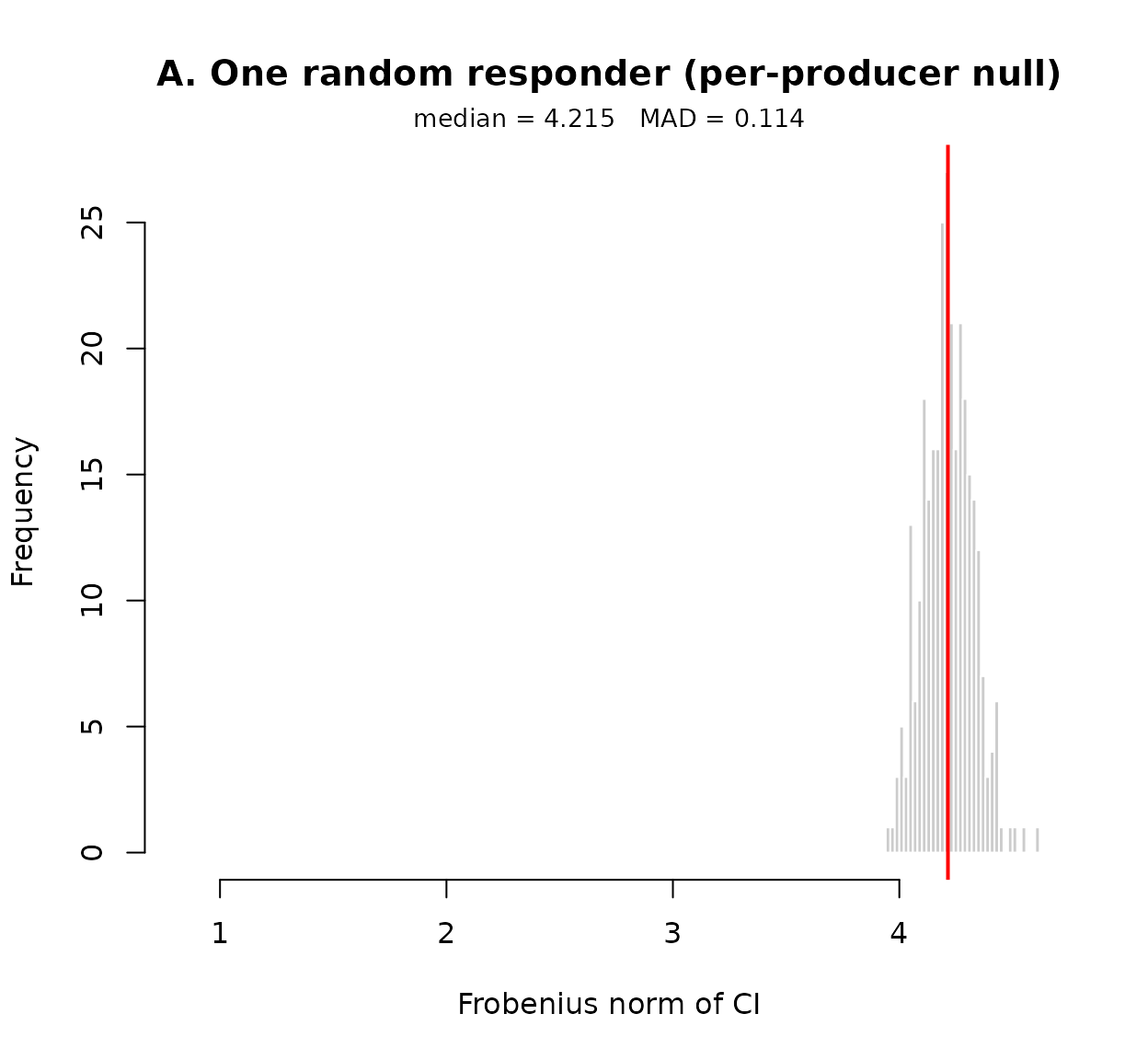
Reference distributions for the per-producer and group-mean nulls, built on the same synthetic noise matrix (1024 pixels, 360-stimulus pool) at 60 trials per producer. Panel A (top): 300 simulated CIs from a single random responder, the reference used by per-producer infoval(). Panel B (bottom): 300 simulated group-mean CIs each built by averaging 20 random responders, the reference used by group_mean_z() at N = 20. Both panels share the x-axis. The bottom distribution sits much closer to zero because averaging cancels independent noise; this 1/sqrt(N) shrinkage is the calibration group_mean_z() uses when scoring the observed group-mean CI.

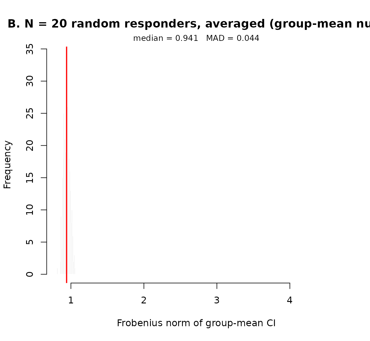
Reference distributions for the per-producer and group-mean nulls, built on the same synthetic noise matrix (1024 pixels, 360-stimulus pool) at 60 trials per producer. Panel A (top): 300 simulated CIs from a single random responder, the reference used by per-producer infoval(). Panel B (bottom): 300 simulated group-mean CIs each built by averaging 20 random responders, the reference used by group_mean_z() at N = 20. Both panels share the x-axis. The bottom distribution sits much closer to zero because averaging cancels independent noise; this 1/sqrt(N) shrinkage is the calibration group_mean_z() uses when scoring the observed group-mean CI.

The same logic applies under real noise matrices. The exact shrinkage factor depends on the noise structure (the synthetic noise above is iid standard normal; real sinusoidal-noise CIs also shrink, just with a different constant), but the qualitative picture (wide distribution in panel A, tight distribution near zero in panel B) survives. The observed group-mean CI’s Frobenius norm is what gets compared against the red median line in panel B. group_mean_z() returns how many MADs above that median the observation sits.

11.5 Why group_mean_z() is not part of the library?

The function is offered only through infoval_report() (as the group_mean_z_unmasked and group_mean_z_masked scalars on its returned data list). Two reasons. First, the inputs that make the reference calibration correct (a noise matrix in raw producers-by-stimulus form, plus a named integer vector of per-producer trial counts) are awkward to assemble outside the infoval_report() pipeline. Second, exposing the function as a public entry point would invite people to read its output as the group-level number, which is exactly the framing this section is asking you to avoid. If you want the statistic, run infoval_report() and pull data$group_mean_z_unmasked or data$group_mean_z_masked; if you want the full Monte-Carlo machinery in a different context, calling infoval() on a single group-CI column with the right trial_counts (the sum of the producer trial counts in the group, per §10’s group-CI recipe) returns the analogous comparison built from the per-producer engine.

12. Agreement maps and publication-ready figures

Three composable plot surfaces share one base-overlay convention: plot_agreement_map() shows the per-pixel one-sample t (signed or |t|), plot_ci_overlay() shows the producer-mean CI (signed), and the cluster-test plot method shows between-condition t-maps. All three accept a base_image argument with the same semantics, so any of them can be rendered as a flat panel or composited on the base face with one call.

12.1 agreement_map_test()

Within a single condition, tests at each pixel whether the producer-level signal differs from zero (one-sample t). The null is built by random sign-flip per producer (exact under the assumption that, under H0, the producer’s signal is symmetric around zero). Family-wise error is controlled by the maximum |t| statistic across pixels.

The agreement statistic. Let $S_{ij}$ be the (raw) signal value at pixel $i$ for producer $j$, with $j = 1, \dots, N$ producers in the condition and $i = 1, \dots, P$ in-mask pixels. The per-pixel one-sample t-statistic is

$$t_i \,=\, \frac{\bar{S}_i}{s_i \,/\, \sqrt{N}}, \qquad \bar{S}_i \,=\, \frac{1}{N} \sum_{j=1}^{N} S_{ij}, \qquad s_i^2 \,=\, \frac{1}{N-1} \sum_{j=1}^{N}\left(S_{ij} - \bar{S}_i\right)^2.$$

What the formula says, pixel by pixel: line up the $N$ producers at the same pixel $i$, treat their signal values $S_{1i}, S_{2i}, \dots, S_{Ni}$ as $N$ numbers, and ask the standard one-sample question “is their mean different from zero?” In words:

• $\bar S_i$ is the average of the producers’ values at pixel $i$. If everyone has slightly positive values there, $\bar S_i$ is a small positive number. If half are positive and half are negative, $\bar S_i$ is near zero.
• $s_i$ is the standard deviation of those values, i.e. how much producers disagree with each other at that pixel.
• $s_i / \sqrt{N}$ is the standard error of the mean: the same amount of disagreement gets damped down once you average over many people, because random noise cancels out as you add more producers.
• $t_i$ divides the average by that standard error. A large $t_i$ means “the producers’ average is far from zero, and they agree with each other about it.” A small $t_i$ means either everyone averaged to roughly zero, or they disagreed wildly so the denominator is large.

A worked example. Imagine $N = 20$ producers and you look at one pixel sitting on the left eyebrow. Say their 20 signal values average to $\bar S_i = 0.30$ with a standard deviation of $s_i = 0.40$. Then $t_i = 0.30 / (0.40 / \sqrt{20}) = 0.30 / 0.089 \approx 3.36$. Across the image you would compute one such $t_i$ for every pixel, producing a map of agreement scores.

The sign of $t_i$ tells you which way the producers agree at pixel $i$: positive means consistently lighter than the base face, negative means consistently darker. The magnitude $|t_i|$ summarises how strongly they agree at that pixel, irrespective of direction. The descriptive agreement map plotted by plot_agreement_map() is this $t_i$ field reshaped to the image grid; the palette = "fire" variant displays $|t_i|$ on a single-hue ramp when only the strength of agreement is needed (see §12.2).

This per-pixel one-sample t against zero is the same logic as the pixel test for smooth classification images introduced by Chauvin, Worsley, Schyns, Arguin, and Gosselin (2005), where a per-pixel z-statistic is computed against the null of no association between noise patterns and responses. The implementation here computes the analogous one-sample t on the per-producer CIs and controls family-wise error using sign-flip permutation in the manner of Maris and Oostenveld (2007) and Nichols and Holmes (2002).

The intuition for sign-flip permutation: under the null hypothesis “this producer’s CI is just noise, with no consistent direction”, the producer’s signal would be just as likely to come out flipped to its mirror image. So you can simulate the null by literally flipping the sign of each producer’s CI independently at random (multiplying their whole CI by $-1$ or $+1$), recomputing $t_i$ at every pixel from the flipped sample, and recording the largest $|t^*_i|$ in that resampled map:

$$T^*_b \,=\, \max_{i'} |t^*_{i'}| \quad \text{on permutation } b.$$

Repeat for $B$ permutations (e.g. $B = 5000$). You now have a null distribution of “biggest agreement that random sign-flipping could produce across the whole image”. Each observed pixel’s p-value is

$$p_i \,=\, \Pr\!\left(\,T^* \,\geq\, |t_i|\,\right),$$

i.e. the fraction of permutations whose image-wide maximum $|t|$ equalled or exceeded the actual $|t_i|$ at pixel $i$.

Why the maximum across pixels, not pixel-by-pixel? With thousands of pixels tested simultaneously, some pixels would clear an uncorrected threshold (e.g. $|t| > 1.96$) by chance even with no real signal. Calibrating each pixel against the maximum statistic over all pixels in random data is the standard family-wise error rate (FWER) fix for spatially correlated maps (Nichols & Holmes, 2002; Maris & Oostenveld, 2007): it guarantees that the probability of even one false-positive pixel under H0 is bounded by $\alpha$. Pixels with $p_i < \alpha$ (default $\alpha = 0.05$) survive the correction.

am <- agreement_map_test(signal_matrix,
                         n_permutations = 5000L,
                         alpha          = 0.05,
                         mask           = make_face_mask(c(256L, 256L)),
                         seed           = 1L)
am$significant_mask  # logical vector: which pixels survive FWER

The result has its own plot() method that renders the observed t-map with FWE-significant pixels outlined in black. This is the one-call form of the standard pairing; see §12.2 for what it does and the color conventions it inherits.

12.2 plot_agreement_map() and plot(agreement_map_test_result)

Renders the per-pixel one-sample t-map as a color image, with optional thresholding and an optional base-face overlay:

# Flat panel.
plot_agreement_map(signal_matrix,
                   img_dims  = c(256L, 256L),
                   threshold = 2.0,
                   palette   = "diverging")

# Same map composited on the base face (recommended for figures).
plot_agreement_map(signal_matrix,
                   img_dims   = c(256L, 256L),
                   threshold  = 2.0,
                   palette    = "diverging",
                   base_image = "data/base.jpg",
                   alpha_max  = 0.7)

On the default diverging palette, both deep red and deep blue indicate strong producer agreement; only the direction differs (blue = producers consistently added to the base, red = consistently subtracted). “No agreement” is the neutral color (white), not red.

If the question is “where do producers have any consistent opinion” rather than “in which direction do they agree”, pass palette = "fire" for a single-hue |t| view (pale yellow at low |t| -> deep red at large |t|). This drops the sign channel by design; the default diverging palette stays preferable when direction matters. To recover direction at a region of interest from a "fire" map, re-render the same data with palette = "diverging" or pair with plot_ci_overlay() of the group-mean CI.

For the inferential variant in one call, pass the agreement_map_test() result straight to plot(). The method reads observed_t, significant_mask, and img_dims from the result, so the source signal_matrix does not need to be re-threaded:

plot(am,
     threshold  = 2.0,
     base_image = "data/base.jpg",
     palette    = "diverging")  # FWE-significant pixels outlined

12.3 plot_ci_overlay()

The headline figure for most papers. Renders the group-mean CI as a translucent layer over the base face, optionally restricted to the significant-pixel mask returned by agreement_map_test() or tracing its boundary as black contours:

plot_ci_overlay(
  signal_matrix,
  base_image = "data/base.jpg",
  test       = am,            # contours significant pixels
  alpha_max  = 0.7
)

plot_agreement_map() and plot_ci_overlay() are cognate surfaces: the agreement map shows the inferential t-statistic (signed or |t|), the CI overlay shows the producer-mean signal (signed), and both can be composited on the same base face. Use the agreement map when the question is “where do producers agree”; use the CI overlay when the question is “what does the group mean look like in the face”.

12.4 plot_dissimilarity_grid()

Lays out multiple rel_dissimilarity() results side-by-side as labelled CI bars. Useful for paper figures showing whether two contrasts have overlapping CIs without forcing the reader to read four numbers from a table:

d_AB <- rel_dissimilarity(sm_a, sm_b, seed = 1L)
d_AC <- rel_dissimilarity(sm_a, sm_c, seed = 1L)

plot_dissimilarity_grid(
  "Trust vs Dominant"  = d_AB,
  "Trust vs Competent" = d_AC,
  metric = "euclidean_normalised"
)

12.5 plot_ci_correlogram()

A publication-ready Pearson-r matrix across multiple group-mean CIs. The function takes a single matrix where each column is one CI (a group mean, an individual producer, or any mix; see §7.5 for the cbind() recipe that mixes per-producer and group CIs in one call). Useful as a compact visual summary of which conditions covary across the image.

Build the input matrix outside the call. Column names become the panel labels.

# trust_cis, friendly_cis, ... are the outputs of
# ci_from_responses_briefrc() or ci_from_responses_2ifc() for
# each condition (see sections 6.1 and 1.3). Each $signal_matrix
# has one column per producer; rowMeans() averages those columns
# into one group-level CI vector. cbind() stacks the per-condition
# group CIs side by side.
ci_matrix <- cbind(
  Trust     = rowMeans(trust_cis$signal_matrix),
  Friendly  = rowMeans(friendly_cis$signal_matrix),
  Competent = rowMeans(competent_cis$signal_matrix),
  Dominant  = rowMeans(dominant_cis$signal_matrix)
)

plot_ci_correlogram(
  ci_matrix,
  mask     = "face",       # also "none", "upper_face", "lower_face"
  triangle = "upper",      # also "full", "lower"
  palette  = "diverging",  # also "diverging_puor", "diverging_brbg"
  file     = "fig3.pdf"    # also "fig3.png" (600 dpi); omit to plot only
)

You can mix group CIs with individual producers by stacking extra columns:

ci_matrix <- cbind(
  Trust_group = rowMeans(trust_cis$signal_matrix),
  Trust_P05   = trust_cis$signal_matrix[, "P05"],
  Trust_P12   = trust_cis$signal_matrix[, "P12"]
)
plot_ci_correlogram(ci_matrix)

When the producers across conditions all live in one signal matrix and the same responses data frame carries the condition column, group_ci() is the shorter path to the same matrix:

# `all_cis$signal_matrix` has one column per producer (named with
# the producer ids); `responses` carries the condition column.
gcis <- group_ci(all_cis$signal_matrix, responses, by = "condition")
plot_ci_correlogram(gcis)

Same diverging convention as the rest of the package’s direction-bearing plots: positive r = blue, negative = red; saturation encodes magnitude. The color scale is fixed at c(-1, 1) so panels are comparable across runs and across paper figures. The §14.6 worked example uses this function on the four-trait subset.

Read the result carefully: Pearson r between two base-subtracted CIs has a positive chance baseline from shared image-domain structure (face shape, signal support); a high absolute r does not by itself license a similarity claim. Use the correlogram for relative comparisons (which pairs covary more than others) rather than absolute claims. For a baseline-free magnitude summary, pair with rel_dissimilarity().

12.6 plot_ci_distance_matrix()

A publication-ready Euclidean distance matrix across multiple group-mean CIs. Same input format as plot_ci_correlogram(): one matrix with one CI per column, individual or group or any mix (the §7.5 cbind() recipe applies here too). Uses the magnitude metric recommended by §9.3 instead of Pearson correlation, with the same Euclidean-distance formula defined there ($D(A, B) = \sqrt{\sum_{i \in \mathcal{M}} (\bar{A}_i - \bar{B}_i)^2}$; the method = "normalised" branch divides by $\sqrt{|\mathcal{M}|}$). Useful when the question is “how far apart are these CIs in pixel space?” rather than “how do they covary?”.

# Same `ci_matrix` constructed in section 10.5: one column per
# group CI, built with cbind() of rowMeans() over each condition's
# per-producer signal matrix.
ci_matrix <- cbind(
  Trust     = rowMeans(trust_cis$signal_matrix),
  Friendly  = rowMeans(friendly_cis$signal_matrix),
  Competent = rowMeans(competent_cis$signal_matrix),
  Dominant  = rowMeans(dominant_cis$signal_matrix)
)

plot_ci_distance_matrix(
  ci_matrix,
  mask     = "face",        # also "none", "upper_face", "lower_face"
  method   = "normalised",  # also "raw" (default); normalised divides
                            # by sqrt(n_pixels_used) for cross-mask
                            # comparability
  triangle = "upper",       # also "full", "lower"
  palette  = "viridis",     # also "inferno", "plasma", "rocket"
  file     = "fig_distance.pdf"
)

Distance is non-negative and unbounded, so the color scale adapts to the data range (unlike the correlogram’s fixed c(-1, 1)). Pale yellow at small distances, deep dark at large distances. The returned object exposes both $distance_matrix (raw or normalised per method) and $distance_raw (always raw, useful for downstream hclust() or MDS).

12.7 plot_ci_mds()

Projects multiple CIs into a low-dimensional Euclidean scatter where distances between points reproduce the Euclidean distances between CIs as faithfully as the chosen number of dimensions allows. Useful for spotting clusters of similar conditions and for showing the relative positions of many group means in one figure.

By default the function fits classical MDS at k = 2, 3, ..., k_max (default k_max = 4) and picks the smallest k whose Kruskal stress-1 against the original distances falls at or below stress_threshold (default 0.05, Kruskal’s “good” interpretive band). When the auto-selected k > 2, the figure becomes a grid of all choose(k, 2) pairwise dimension panels so no information is hidden by a premature flattening to 2D.

Kruskal’s (1964) interpretive bands for stress-1:

• 0.025 excellent (the kD map is essentially exact)
• 0.05 good (small distortions; safe to interpret)
• 0.10 fair (interpret carefully; check the trace)
• 0.20 poor (the projection is hiding more than it shows)
• > 0.20 very poor

# Build a CI matrix the same way as for the correlogram: one
# column per group CI.
ci_matrix <- cbind(
  Trust      = rowMeans(trust_cis$signal_matrix),
  Friendly   = rowMeans(friendly_cis$signal_matrix),
  Competent  = rowMeans(competent_cis$signal_matrix),
  Dominant   = rowMeans(dominant_cis$signal_matrix),
  Submissive = rowMeans(submissive_cis$signal_matrix)
)

# Minimal call: auto-selects k, prints a one-screen summary.
out <- plot_ci_mds(ci_matrix, mask = "face")
print(out)            # one-screen view of dimensionality selection

# The coordinates of each CI in the Euclidean MDS space:
out$mds_points

# Per-k stress (was the auto-choice sensible?):
out$stress_by_k

# A grouped scatter for a multi-condition design. `groups`
# colors points; `shapes` adds a second categorical level.
# `country_codes` and `trait_family` are character vectors with
# one entry per column of `ci_matrix_country_trait` (built the
# same cbind() way as above). Force a single 2D paper panel
# once fidelity has been audited.
plot_ci_mds(
  ci_matrix_country_trait,
  mask     = "face",
  k        = 2L,
  groups   = country_codes,
  shapes   = trait_family,
  file     = "fig_mds.pdf"
)

See §9.3 for rel_dissimilarity() (the two-condition Euclidean distance with bootstrap CI) and §12.6 for the all-vs-all distance matrix plot_ci_mds() projects internally.

13. Region-restricted analyses

Every rel_*() and infoval() accepts a mask argument. When you supply one:

• rel_*() row-subsets the signal matrix to the masked pixels before computing the statistic. The reported n_pixels reflects the subsetted count.
• rel_cluster_test() uses a zero-out pattern instead, setting per-pixel t to 0 outside the mask. This preserves the 2D image structure required for 4-connectivity and TFCE.
• infoval() applies the mask symmetrically to both the observed Frobenius norm and the reference distribution.
• agreement_map_test() row-subsets and embeds the result back into a full-image vector (NA outside the mask).

The same mask object should pass through all metrics in a single analysis. Mixing masked observed values with an unmasked reference yields a number with no defensible interpretation. To compare across regions, run the metric once per mask:

for (region in c("eyes", "nose", "mouth",
                 "upper_face", "lower_face")) {
  m <- make_face_mask(c(256L, 256L), region = region)
  cat(region, ": ICC(3,1) =",
      rel_icc(signal_matrix, mask = m)$icc_3_1, "\n")
}

14. Worked example on real dataset

This section runs the package end-to-end on a published 2IFC dataset. The original paper reports the per-trait classification images and judge ratings. The reliability, discriminability, infoVal, and region-restricted analyses below are new and extend that work; the package post-dates the paper. Numbers and figures below come from running the package on the open data.

Oliveira, M., Garcia-Marques, T., Dotsch, R., & Garcia-Marques, L. (2019). Dominance and competence face to face: Dissociations obtained with a reverse correlation approach. European Journal of Social Psychology. https://doi.org/10.1002/ejsp.2569. Open data: https://doi.org/10.17605/osf.io/hr5pd.

In Study 1, 200 participants completed a 2IFC reverse-correlation task with 300 trials each on a 256 x 256 grayscale male base face, across 10 trait conditions in a between-subjects design (20 producers per trait): Dominant, Submissive, Trust, Untrust, Friendly, Unfriendly, Intelligent, Unintelligent, Competent, Incompetent.

The R code chunks below are shown for reading and adaptation. The numbers and figures alongside each chunk were computed on the open OSF data for this study. Copy the chunks into a fresh R session and run them on your own data to reproduce the analysis pattern.

14.1 Loading the data

The original CSV is semicolon-separated. We read it with read.csv2(), then rename subject to the column name the package expects, store the ids as text (so they are not treated as numeric), and lower-case the trait labels for consistency:

library(rcisignal)

raw <- read.csv2("study1data.csv", stringsAsFactors = FALSE)
raw$participant_id <- as.character(raw$subject)
raw$trait          <- tolower(raw$trait)
raw <- raw[, c("participant_id", "trial",
               "stimulus", "response", "trait")]

head(raw)
#>   participant_id trial stimulus response trait
#> 1           8001     1      152        1  dominant
#> 2           8001     2      284       -1  dominant
#> 3           8001     3      176        1  dominant
#> ...

14.2 Modernizing the legacy rcicr 0.3.0 rdata

The 2015 rdata stores its noise basis under s$sinusoids and s$sinIdx; current rcicr expects p$patches and p$patchIdx. Patch the legacy file without re-running stimulus generation:

load("rcic_seed_1_time_fev_05_2015_03_17.Rdata")  # legacy file

p <- list(
  patches    = s$sinusoids,
  patchIdx   = s$sinIdx,
  noise_type = "sinusoid"
)

save(list = ls(), file = "stimuli_modernised.RData")

The new stimuli_modernised.RData is the file the package will read.

14.3 Diagnostics

The diagnostic battery runs in one call:

report <- run_diagnostics(
  raw[, c("participant_id", "stimulus", "response")],
  method     = "2ifc",
  rdata      = "stimuli_modernised.RData",
  expected_n = 300L
)
print(report)

On this dataset, the report’s summary is:

check	status	label
response_coding	pass	Response coding
trial_counts	pass	Trial counts
duplicates	pass	Duplicates
response_bias	pass	Response bias
stimulus_alignment	pass	Stimulus alignment
version_compat	warn	rcicr version compatibility

The version warning (when present) is informational and expected on this dataset because the experiment was run with rcicr 0.3.x in 2015. The basic mechanics are clean.

Some research designs cross multiple conditions, in which case running check_response_bias() separately per condition is useful (a producer who looks balanced overall may still be heavily biased in one trait):

trait_bias <- list()
for (tr in sort(unique(raw$trait))) {
  sub <- subset(raw, trait == tr,
                c("participant_id", "stimulus", "response"))
  trait_bias[[tr]] <- check_response_bias(sub, method = "2ifc")
}
trait_bias[["competent"]]

For this dataset, all ten trait conditions return PASS.

14.4 Per-trait infoVal

infoval() reports a per-producer Frobenius-norm z-score against a trial-count-matched reference. Running it on each of the ten trait conditions, masked with the package’s default full-face oval, gives the table below:

Trait	Median producer z	n above 1.96 (of 20)	Group-mean z
competent	+0.70	3	+3.03
dominant	+0.89	6	+7.09
friendly	+0.97	5	+18.50
incompetent	+0.59	2	+2.13
intelligent	+0.67	3	+8.23
submissive	+0.37	5	+3.78
trust	+0.50	3	+11.95
unfriendly	+0.85	5	+15.73
unintelligent	+0.63	3	+2.03
untrust	+0.84	7	+9.58

Group-mean z is the headline. Per-producer median z sits well below 1.96 across all ten conditions, while the group-mean z typically clears it. This pattern is structural rather than a data problem: per-producer Frobenius norms aggregate over the whole image and dilute localised signal, so individual z values are systematically smaller than the group-mean equivalent on the same data.

14.5 Building the per-trait signal matrices

The package builds the signal matrix for one trait in a single call. The output is a list whose $signal_matrix is what every downstream metric needs:

trust_trials <- raw[raw$trait == "trust", ]
trust_cis    <- ci_from_responses_2ifc(
  trust_trials,
  rdata_path = "stimuli_modernised.RData",
  base_image  = "male"
)
trust_cis$signal_matrix     # n_pixels x n_producers

To get signal matrices for all ten traits at once, loop the call and collect the results in a named list:

traits    <- sort(unique(raw$trait))
sm        <- vector("list", length(traits))
names(sm) <- traits

for (tr in traits) {
  cis      <- ci_from_responses_2ifc(
    raw[raw$trait == tr, ],
    rdata_path = "stimuli_modernised.RData",
    base_image  = "male"
  )
  sm[[tr]] <- cis$signal_matrix
}

# A few convenience aliases for the contrasts used below.
sm_trust     <- sm[["trust"]]
sm_dominant  <- sm[["dominant"]]
sm_competent <- sm[["competent"]]
sm_friendly  <- sm[["friendly"]]

sm is now a named list of ten signal matrices, each 65,536 x 20 (n_pixels x n_producers). The contrasts and metrics in the sections that follow use these matrices directly. If you want a detailed walkthrough of how the function builds the per-producer mask, the four-step recipe in §3.3 walks it through.

14.6 Within-condition reliability per trait

run_reliability() returns split-half (with Spearman-Brown projection) and ICC(3,*) on a single signal matrix. Run it on each per-trait signal matrix:

rel_table <- data.frame(trait = traits,
                        r_sb = NA_real_, icc_3_k = NA_real_)
for (i in seq_along(traits)) {
  rep <- run_reliability(sm[[traits[i]]],
                         n_permutations = 2000L,
                         seed = 1L, progress = FALSE)
  rel_table$r_sb[i]    <- rep$results$split_half$r_sb
  rel_table$icc_3_k[i] <- rep$results$icc$icc_3_k
}
rel_table

On this dataset, the resulting table is:

Trait	r_sb	ICC(3,1)	ICC(3,k)
competent	0.31	0.02	0.30
dominant	0.52	0.05	0.51
friendly	0.82	0.18	0.81
incompetent	0.20	0.01	0.19
intelligent	0.55	0.06	0.54
submissive	0.30	0.02	0.29
trust	0.69	0.10	0.69
unfriendly	0.75	0.13	0.74
unintelligent	0.25	0.02	0.24
untrust	0.62	0.07	0.61

Spearman-Brown projected reliabilities and ICC(3,k) values are high throughout, indicating that the group-level CIs are stable across producer halves.

Cross-trait CI correlations

Restricted to the four traits used in the example contrasts (trust, friendly, competent, dominant), pairwise Pearson correlations between the group-mean CIs follow the expected valence structure: prosocial pairs correlate positively (trust–friendly +0.68, friendly–competent +0.48, trust–competent +0.42), and pairs that cross into dominance correlate negatively (friendly–dominant −0.50, trust–dominant −0.37). Competent–dominant is weakly negative (−0.22).

Correlations are computed over the pixels inside the parametric oval face mask (make_face_mask(c(256L, 256L), region = "full")), matching the masking step described in Oliveira et al. (2019, p. 892). Without the mask, off-face pixels carry sinusoid energy from the noise pool and attenuate every pair by roughly 0.02–0.05. The full ten-trait matrix reproduces Oliveira et al. (2019) Table 2 to within ±0.02 across all spot-checked cells.

	trust	friendly	competent	dominant
trust		+0.68	+0.42	-0.37
friendly			+0.48	-0.50
competent				-0.22
dominant

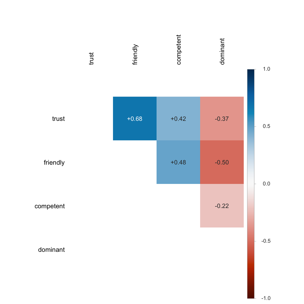
Pairwise Pearson correlations between the four group-mean CIs (trust, friendly, competent, dominant) in the Oliveira et al. (2019) Study 1 data. Diverging palette; blue = positive, red = negative; saturation indicates magnitude. Lower triangle and diagonal omitted because they are redundant.

Cross-trait distances (Euclidean)

Per §9.3, Pearson r between base-subtracted CIs carries a positive baseline from shared image-domain structure and is not a clean similarity score; Euclidean distance does not share this baseline issue. plot_ci_distance_matrix() produces the companion magnitude view on the same four traits:

# `sm` is the named list of ten per-trait signal matrices built
# in §14.5. `plot_ci_distance_matrix()` reduces each matrix to
# its group mean internally; no manual averaging is needed.
plot_ci_distance_matrix(
  list(Trust     = sm[["trust"]],
       Friendly  = sm[["friendly"]],
       Competent = sm[["competent"]],
       Dominant  = sm[["dominant"]]),
  img_dims = c(256L, 256L),
  mask     = "face",
  method   = "raw",        # "normalised" for cross-mask comparability
  triangle = "upper"
)

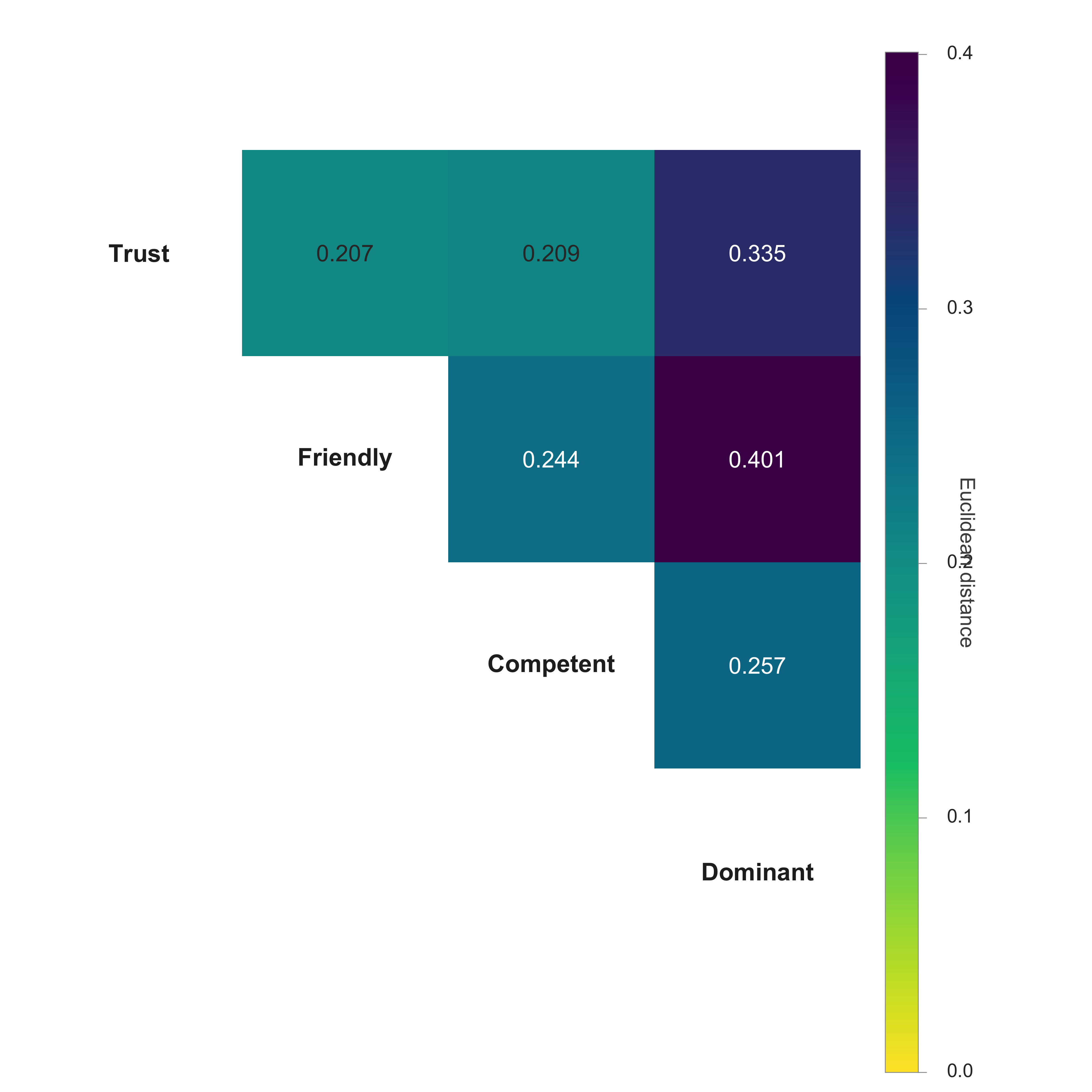
Pairwise Euclidean distances between the same four group-mean CIs, restricted to the face oval. Sequential viridis palette: pale yellow at small distances, deep purple at large distances. Cell values are raw distances in CI units. The ordering mirrors the correlation story (prosocial pairs closer; pairs crossing into dominance farther apart) but on a baseline-free magnitude scale.

Pairs that the correlogram flagged as prosocially-aligned (Trust–Friendly, Trust–Competent, Friendly–Competent) sit at distances 0.21–0.24, while Friendly–Dominant tops the matrix at 0.40. Same qualitative story, no positive-baseline confound.

Trait-CI map (MDS on all 10 conditions)

plot_ci_mds() projects all ten conditions into a low- dimensional Euclidean scatter where distances between points reproduce the pairwise distances between CIs as faithfully as the chosen number of dimensions allows. By default the function fits classical MDS at every k from 2 to k_max and auto- selects the smallest k whose Kruskal stress-1 reaches the “good” band (0.05). When the data have a theoretical reason to be plotted in a specific number of dimensions, for example, a two-axis hypothesis like warmth vs dominance, pass an integer k to override the auto-selection.

The Oliveira et al. (2019) trait-rating literature works with a two-dimensional theoretical structure (warmth and competence families, with dominance as a separate axis when split). The 2D paper figure for that hypothesis uses k = 2L:

# `sm` is the named list of ten per-trait signal matrices built
# in §14.5. Pick the ten traits in display order, then relabel
# them with the pretty (display) names. `plot_ci_mds()` reduces
# per-producer matrices to group means internally, so we pass
# the matrices as-is.
trait_order  <- c("trust",     "friendly",   "untrust",   "unfriendly",
                  "competent", "intelligent","incompetent","unintelligent",
                  "dominant",  "submissive")
trait_pretty <- c("Trust",     "Friendly",   "Untrust",   "Unfriendly",
                  "Competent", "Intelligent","Incompetent","Unintelligent",
                  "Dominant",  "Submissive")
trait_family <- c("warmth", "warmth", "warmth", "warmth",
                  "competence", "competence", "competence", "competence",
                  "dominance", "dominance")
trait_pole   <- c("positive", "positive", "negative", "negative",
                  "positive", "positive", "negative", "negative",
                  "positive", "negative")

mds_input        <- sm[trait_order]
names(mds_input) <- trait_pretty

plot_ci_mds(
  mds_input,
  img_dims = c(256L, 256L),
  mask     = "face",
  k        = 2L,             # theory-driven: 2D paper figure
  groups   = trait_family,   # warmth / competence / dominance
  shapes   = trait_pole      # positive / negative pole
)

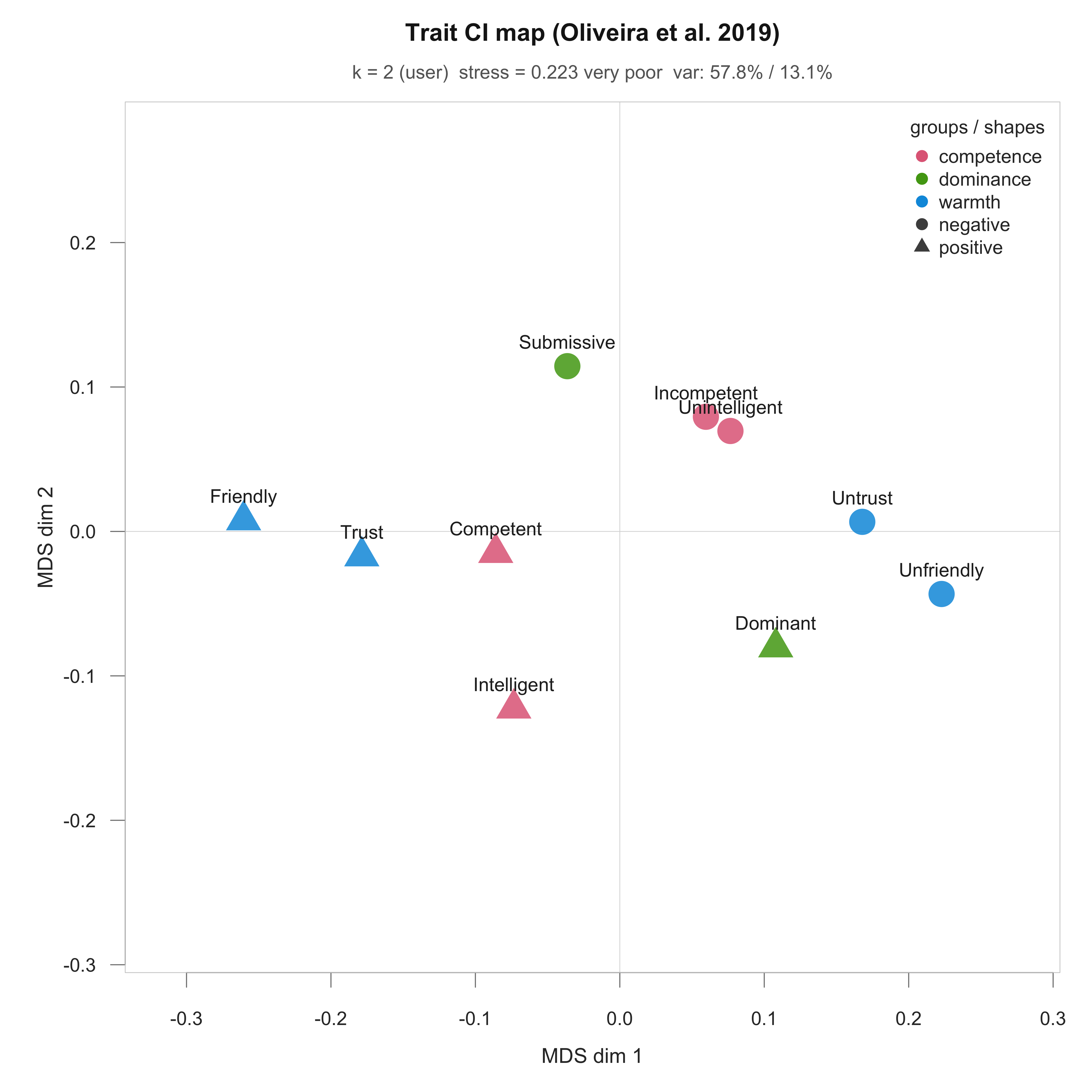
Classical MDS projection of all ten trait CIs in the Oliveira et al. (2019) data, fit to face-masked raw Euclidean distances and forced to k = 2 dimensions for theory-driven plotting. The Kruskal stress at k = 2 is 0.223 (Kruskal’s ‘very poor’ band); the first two axes capture 57.8% and 13.1% of the absolute eigenmass. Points color by trait family (warmth / dominance / competence); triangles mark the positive pole within each family, circles the negative pole.

Three reading notes.

First, the GOF header reports k = 2 (user) stress = 0.223 very poor. Forcing 2D here means accepting Kruskal’s “very poor” band; the 2D projection genuinely distorts the underlying distance structure. The auto-selector would have escalated to k = k_max = 4 and rendered a 6-panel pair-grid because no tested k reaches the “good” threshold (stress at k=3 is 0.175, at k=4 is 0.142, all “poor”). The theory-driven 2D figure is the right paper figure when the hypothesis is two-dimensional, but readers should be told what the 2D projection is hiding.

Second, report the per-k stress trace alongside any single- panel MDS figure. For this dataset the trace is

k	stress-1	Kruskal band	cumulative variance
2	0.223	very poor	70.9%
3	0.175	poor	77.7%
4	0.142	poor	83.1%

so the 2D figure preserves 71% of the absolute eigenmass but distorts the distance structure enough to fall in the “very poor” Kruskal band. The 3D and 4D projections recover more fidelity but never reach the “good” threshold within k_max = 4; the trait space in this dataset is genuinely high-dimensional. Interpret point positions in the 2D figure in relative terms (which conditions cluster together, which families separate) rather than as absolute distances.

Third, despite the modest fidelity, the 2D figure recovers intuitive substructure. Warmth-positive traits (Trust, Friendly) sit on the left; warmth-negative (Untrust, Unfriendly) on the right. The competence family (Competent / Intelligent / Incompetent / Unintelligent) occupies the centre, with the positive-pole traits to the left and the negative-pole traits slightly to the right. Dominance is split: Dominant sits on the right with the warmth-negative cluster while Submissive sits on its own at the top. Higher-dimensional projections (k = 3L, k = 4L, or letting auto-selection escalate) separate the competence axis from the warmth axis more clearly, at the cost of more panels to read.

ICC and group-mean infoVal z track each other across traits

Per-trait reliability and per-trait group-mean infoVal z (see §10) are tightly coupled across the ten conditions in this dataset: Pearson r = 0.97, 95% CI [0.88, 0.99], t(8) = 11.41, p < 0.001. Both quantify producer alignment on the pixel-level signal: ICC(3,k) as a variance ratio, group-mean z as the magnitude of the surviving group-mean signal against a matched reference. Conditions where producers converge on a common spatial template (friendly, unfriendly, trust) sit in the upper right; conditions where producer templates are largely idiosyncratic (incompetent, unintelligent) sit in the lower left.

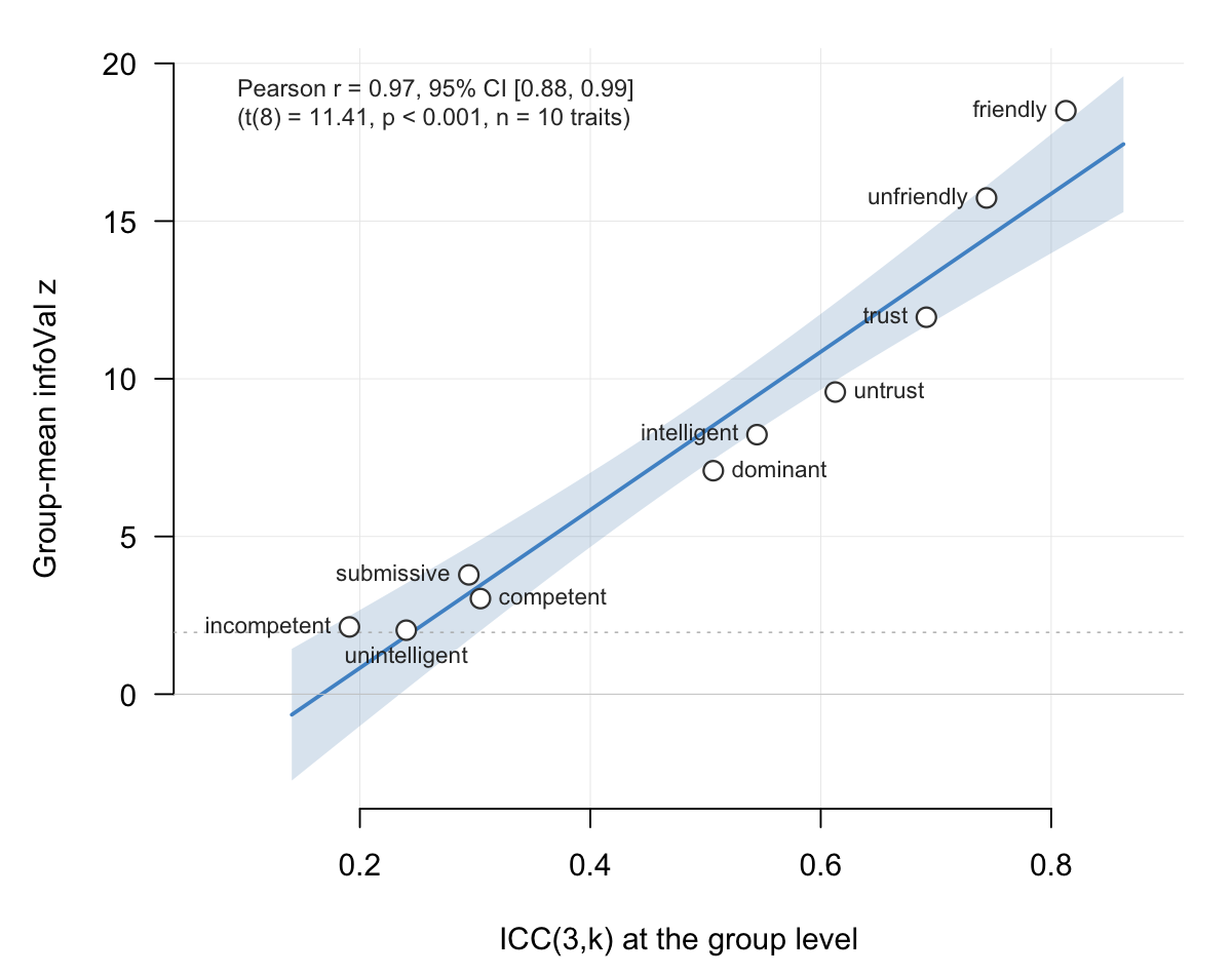
Per-trait ICC(3,k) versus per-trait group-mean infoVal z on the Oliveira et al. (2019) Study 1 data. Each point is one of the ten trait conditions; the line is the OLS fit and the band is its 95% confidence band. The dotted reference line marks group-mean z = 1.96.

14.7 Multi-contrast discriminability (full face)

Three motivating questions you can put to this dataset, going beyond the original paper:

• Trust vs Friendly: two trait labels often grouped under “warmth/morality”. Where do their visual representations diverge?
• Competent vs Dominant: two trait labels conceptually related to ability and agency but with opposite valence (Oliveira et al. 2019). Where on the face do they diverge?
• Trust vs Dominant: a cross-quadrant contrast spanning two functional dimensions, included as a reference benchmark.

Each contrast is a stratified cluster permutation test on the full face. We summarize the overall magnitude of each divergence with rel_dissimilarity() and lay them out side-by-side:

# Three contrasts. Each is a named list with `$a` and `$b`: the
# two per-trait signal matrices to compare. Building it this way
# means the same `contrasts` object can drive both the full-face
# tests below and the region-by-region tests in §14.8.
contrasts <- list(
  "Trust vs Friendly"     = list(a = sm[["trust"]],
                                 b = sm[["friendly"]]),
  "Competent vs Dominant" = list(a = sm[["competent"]],
                                 b = sm[["dominant"]]),
  "Trust vs Dominant"     = list(a = sm[["trust"]],
                                 b = sm[["dominant"]])
)

# Empty named lists to hold one result per contrast.
ct_full     <- vector("list", length(contrasts))
dissim_full <- vector("list", length(contrasts))
names(ct_full)     <- names(contrasts)
names(dissim_full) <- names(contrasts)

# Compute the cluster test and the bootstrap dissimilarity for
# each contrast. One loop pass per contrast; both results go
# into their named slots.
for (cname in names(contrasts)) {
  a <- contrasts[[cname]]$a
  b <- contrasts[[cname]]$b

  ct_full[[cname]] <- rel_cluster_test(
    a, b,
    img_dims          = c(256L, 256L),
    cluster_threshold = 2.0,
    n_permutations    = 2000L,
    seed              = 1L,
    progress          = FALSE
  )

  dissim_full[[cname]] <- rel_dissimilarity(
    a, b,
    n_boot         = 2000L,
    null           = "permutation",
    n_permutations = 2000L,
    seed           = 1L,
    progress       = FALSE
  )
}

# Side-by-side bootstrap-CI display of all three contrasts.
plot_dissimilarity_grid(
  "Trust vs Friendly"     = dissim_full[["Trust vs Friendly"]],
  "Competent vs Dominant" = dissim_full[["Competent vs Dominant"]],
  "Trust vs Dominant"     = dissim_full[["Trust vs Dominant"]]
)

On this dataset, the dissimilarity grid is:

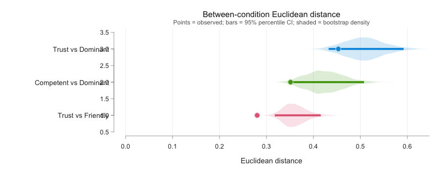
Between-condition Euclidean distance for the three contrasts on the Oliveira et al. (2019) Study 1 data. Each row is one contrast. The white-bordered point is the observed Euclidean distance between the two group-mean CIs, computed across all 65,536 pixels of the 256 x 256 image. The bar around it is the 95% percentile bootstrap CI from 2000 producer-level resamples (each condition resampled independently with replacement, distance recomputed on the resample). The shaded silhouette is the kernel density of the bootstrap distribution, scaled to the row height for visual comparison; its width does not encode units. Larger values mean the two group CIs sit farther apart in pixel space. The bar shows how precisely each distance is estimated under producer resampling; because resampling biases the distance upward, a bar clear of zero is not itself a test of difference. The above-chance test is the permutation null reported in the table below.

The bootstrap bars in the figure show the precision of each distance estimate under producer resampling; because that resampling biases the distance upward, a bar clear of zero is not by itself evidence of a difference (see the §9.3 callout). The above-chance test is the permutation null, summarised per contrast below:

Contrast	d	M null	SD null	z	d/median	p perm
Trust vs Friendly	0.28	0.23	0.015	+3.0	1.20	0.0040
Competent vs Dominant	0.35	0.25	0.020	+5.2	1.42	0.0005
Trust vs Dominant	0.45	0.25	0.022	+9.4	1.84	0.0005

Each contrast sits in the upper tail of its own permutation null (z from +3.0 to +9.4, all p < .01), so the divergences are larger than the chance distance between two random producer subgroups. That is the claim the bootstrap CI alone cannot support.

14.8 Region-by-region cluster tests

A typical follow-up question is whether the divergences are uniform across the face or driven by specific anatomical regions. Run the cluster test once per region per contrast. The same three contrasts × four regions (full, eyes, mouth, upper face) gives twelve cells, which is small enough to scan as a table:

regions <- c("full", "eyes", "mouth", "upper_face")

cluster_grid <- expand.grid(
  contrast = names(contrasts),
  region   = regions,
  stringsAsFactors = FALSE
)
cluster_grid$n_clusters    <- NA_integer_
cluster_grid$n_significant <- NA_integer_
cluster_grid$min_p         <- NA_real_

for (i in seq_len(nrow(cluster_grid))) {
  cname  <- cluster_grid$contrast[i]
  region <- cluster_grid$region[i]
  m  <- make_face_mask(c(256L, 256L), region = region)
  ct <- rel_cluster_test(
    contrasts[[cname]]$a, contrasts[[cname]]$b,
    img_dims          = c(256L, 256L),
    mask              = m,
    cluster_threshold = 2.0,
    n_permutations    = 2000L,
    seed              = 1L,
    progress          = FALSE
  )
  cl <- ct$clusters
  cluster_grid$n_clusters[i]    <- if (is.null(cl)) 0L else
    nrow(cl)
  cluster_grid$n_significant[i] <-
    sum(cl$significant, na.rm = TRUE)
  cluster_grid$min_p[i]         <-
    if (is.null(cl) || nrow(cl) == 0L) NA_real_ else
      min(cl$p_value, na.rm = TRUE)
}

cluster_grid

On this dataset, the resulting grid is:

Contrast	Region	n clusters	n significant	min p
Trust vs Friendly	full	220	1	0.0430
Competent vs Dominant	full	223	3	0.0045
Trust vs Dominant	full	243	6	0.0000
Trust vs Friendly	eyes	83	0	0.2450
Competent vs Dominant	eyes	82	2	0.0150
Trust vs Dominant	eyes	101	4	0.0010
Trust vs Friendly	mouth	9	0	0.0630
Competent vs Dominant	mouth	10	2	0.0065
Trust vs Dominant	mouth	10	1	0.0200
Trust vs Friendly	upper_face	118	0	0.3115
Competent vs Dominant	upper_face	115	1	0.0185
Trust vs Dominant	upper_face	150	5	0.0050

The pattern of significant clusters across regions tells you where on the face each pair of conditions diverges and how strongly the producer sample agreed on those divergences (via FWER-controlled permutation). When a contrast shows a large full-face cluster but no significant clusters in any single region, the divergence is broad rather than localised; when the opposite holds, you have evidence for a localised contrast driven by one anatomical area.

14.9 Per-region informational value

Per-producer informational value also varies by region. A trait whose group CI looks weak overall may carry stronger signal in one specific region, and vice versa. Run infoval() per region per condition:

# 2IFC reference pool, reconstructed once from the modernised rdata
# (the same file the signal matrices were built from in 14.5).
noise_matrix <- read_noise_matrix("stimuli_modernised.RData",
                                  base_image = "male")

iv_grid <- expand.grid(
  trait  = c("trust", "friendly", "competent", "dominant"),
  region = regions,
  stringsAsFactors = FALSE
)
iv_grid$median_z <- NA_real_
iv_grid$n_above  <- NA_integer_

for (i in seq_len(nrow(iv_grid))) {
  label  <- iv_grid$trait[i]
  region <- iv_grid$region[i]
  sig    <- sm[[label]]                          # per-trait signal matrix
  resp   <- raw[raw$trait == label, ]            # trial-level rows for this trait
  m      <- make_face_mask(c(256L, 256L), region = region)
  iv     <- infoval(sig, noise_matrix,
                    responses = resp,            # infoval derives trial counts
                    iter      = 1000L,
                    mask      = m,
                    seed      = 1L,
                    progress  = FALSE)
  iv_grid$median_z[i] <- stats::median(iv$infoval)
  iv_grid$n_above[i]  <- sum(iv$infoval >= 1.96)
}

iv_grid

On this dataset, the resulting grid is:

Trait	Region	Median producer z	n above 1.96 (of 20)
trust	full	+0.50	3
friendly	full	+0.97	5
competent	full	+0.70	3
dominant	full	+0.89	6
trust	eyes	+0.50	1
friendly	eyes	+0.34	2
competent	eyes	+0.36	2
dominant	eyes	+0.91	3
trust	mouth	+0.53	3
friendly	mouth	+0.75	4
competent	mouth	+0.25	5
dominant	mouth	+0.38	2
trust	upper_face	+0.30	2
friendly	upper_face	+0.23	2
competent	upper_face	+0.21	3
dominant	upper_face	+0.37	5

Compared with the full-face infoVal table in §14.4, this region-restricted view often shifts the picture. A trait whose group CI looks weak overall may carry stronger signal in one specific region, and a trait that looks strong overall may localise to one region rather than spanning the whole face.

In this dataset the regional pattern is informative on its own. Dominance carries comparatively strong signal in the eyes (median producer z noticeably higher than the other three traits in that region) and weaker, comparable signal in the mouth and upper face. Friendliness flips that pattern, with the mouth carrying its strongest regional signal and the upper face its weakest. Trustworthy localises broadly across the eyes and mouth without a clear regional peak, and competent’s signal is the most evenly spread across regions, though at uniformly modest levels. The headline full-face median for each trait masks these regional contrasts.

The two grids (the cluster grid from §14.8 and the infoVal grid here) answer two different questions about the same masked region. The cluster test asks where conditions A and B disagree; infoVal asks how informative a single condition’s mask is when restricted to this region. Reporting both side-by-side gives a fuller picture of how producers’ representations organize across the face.

14.10 Pairwise cluster maps for two motivating contrasts

The two contrasts highlighted in this section are chosen because they sit at opposite ends of a methodological prediction. Trust versus Friendly pits two traits that load on the same warmth dimension of social judgement and share much of their facial encoding, so the expectation is a comparatively narrow set of pixel-level differences. Dominant versus Competent pits two traits that the original paper (Oliveira et al., 2019) argues dissociate: dominance is read off coarser whole-face structure while competence draws on finer ability cues, and the two should therefore diverge over a broader spatial region. The maps below let the reader judge whether the data agree.

For each between-condition contrast we render two complementary maps on the same male base face. The descriptive map shows the difference of the two group-mean CIs across all pixels in the face oval, with no inferential filter applied; it lets the reader see the raw spatial pattern first, before any thresholding is layered on. The FWER-controlled map shows the same difference restricted to pixels inside a cluster significant at p < .05 under FWER-controlled cluster-based permutation testing. Showing both side-by-side lets the reader see how much of the descriptive pattern is supported once a controlled Type I error filter is applied.

For each contrast we (i) take the difference of the two group- mean CIs, (ii) render it on the base face (descriptive view), (iii) run rel_cluster_test() to find spatially contiguous regions where the per-pixel Welch t exceeds the cluster-forming threshold, and (iv) overlay the same difference on the base face restricted to pixels belonging to a significant cluster (2000 stratified label permutations, max-mass null, cluster threshold |t| > 2.0).

# Descriptive map: difference of group means, no significance filter.
# sm[["trust"]] and sm[["friendly"]] are per-producer signal matrices
# (one column per producer); rowMeans() averages the columns down to
# one group-level CI vector per trait.
diff_signal <- rowMeans(sm[["trust"]]) - rowMeans(sm[["friendly"]])

plot_ci_overlay(
  diff_signal,
  base_image = "base.jpg",
  mask       = make_face_mask(c(256L, 256L), region = "full"),
  main       = "Trust minus Friendly (descriptive)"
)

# FWER-controlled map: same difference, masked to significant clusters.
ct_tf <- rel_cluster_test(
  sm[["trust"]], sm[["friendly"]],
  img_dims          = c(256L, 256L),
  cluster_threshold = 2.0,
  n_permutations    = 2000L,
  seed              = 1L
)

# Pull out the cluster ids of the significant clusters in each
# direction (Trust > Friendly = "pos", Friendly > Trust = "neg").
sig_pos <- ct_tf$clusters$cluster_id[ct_tf$clusters$direction == "pos" &
                                     ct_tf$clusters$significant]
sig_neg <- ct_tf$clusters$cluster_id[ct_tf$clusters$direction == "neg" &
                                     ct_tf$clusters$significant]

# Build a logical mask marking pixels that fall inside any
# significant cluster (in either direction). `pos_labels` and
# `neg_labels` are integer matrices of cluster ids; %in% checks
# membership pixel by pixel.
sig_mask <- (ct_tf$pos_labels %in% sig_pos) |
            (ct_tf$neg_labels %in% sig_neg)

# Plot the same diff_signal on the base face, but show it only
# where sig_mask is TRUE (inside a significant cluster).
plot_ci_overlay(
  diff_signal,
  base_image = "base.jpg",
  mask       = as.vector(sig_mask),
  main       = "Trust minus Friendly (FWER-controlled clusters)"
)

Descriptive maps. No significance filter applied; the display is restricted to the face oval so the color scale is not dominated by hair/background pixels.

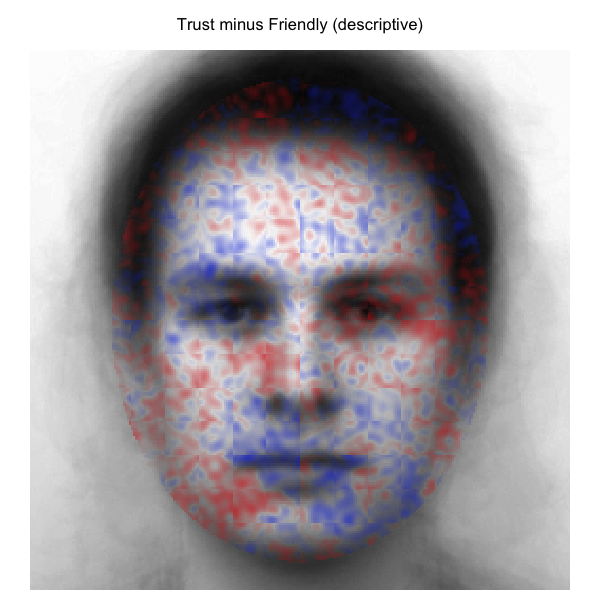
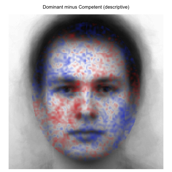
Descriptive pairwise difference maps on the male base face. Left: Trust minus Friendly. Right: Dominant minus Competent. Blue = first condition stronger; red = second condition stronger; opacity = magnitude of the difference. The display covers every pixel in the full-face oval; no inferential filter is applied. These maps show the raw spatial pattern of agreement before any cluster-based permutation testing.

FWER-controlled maps. Same difference signals, but pixels outside any significant cluster appear transparent so the base face shows through.

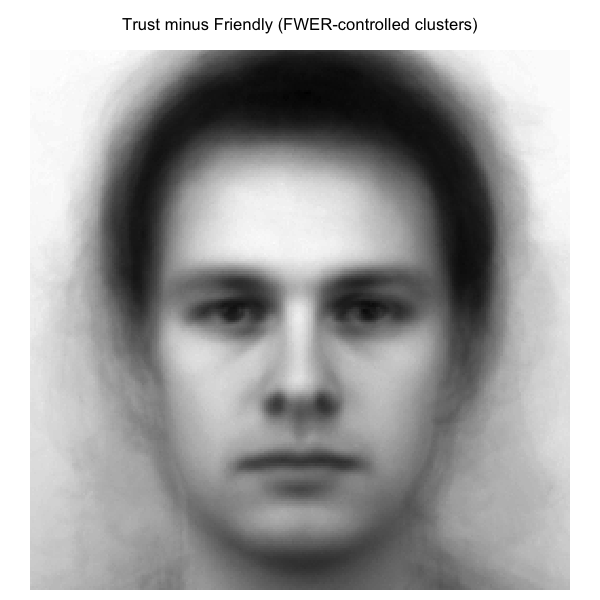
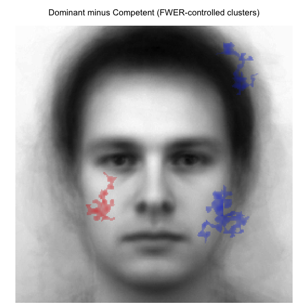
FWER-controlled pairwise cluster-agreement maps on the male base face. Left: Trust minus Friendly. Right: Dominant minus Competent. Each map shows the difference of the two group-mean CIs only at pixels belonging to a cluster that is significant at p < .05 under FWER-controlled cluster-based permutation testing (cluster threshold |t| > 2.0; 2000 stratified label permutations; max-mass null). Color convention as in the descriptive maps above (blue = first condition stronger; red = second condition stronger; opacity = magnitude). Compare with the descriptive maps to see how much of the raw pattern survives the inferential filter.

The two contrasts pick out qualitatively different spatial signatures, broadly consistent with the prediction set out at the start of this section. Trust versus Friendly localises around the eye and mid-face regions, consistent with the warmth dimension being read off socially-relevant features and shared across the two traits. Dominant versus Competent spreads more widely across the face, consistent with a contrast that draws on both whole-face agency cues and finer ability cues. Among the pixels that survive the FWER filter, the Dominant vs Competent map retains noticeably more spatial extent than the Trust vs Friendly map. These maps extend Oliveira et al. (2019) by adding a between-condition inferential filter the original paper did not run.

14.11 Producer agreement maps (within-condition)

The pairwise maps in §14.10 ask where two conditions differ. A complementary question is where, within one condition, do producers agree with each other?. plot_agreement_map() with palette = "fire" answers that visually: at each pixel it runs a one-sample t-test of the per-producer signals against zero, takes the absolute value, and renders |t| on a single-hue ramp. Pale-yellow pixels are places where producers did not consistently push in one direction (low agreement); deep-red pixels are where they pushed strongly and consistently in the same direction (high agreement). The unipolar "fire" view discards sign by design; pair with palette = "diverging" or with plot_ci_overlay() if you also need to know which way the agreement points.

The chunk below renders the four warmth / agency traits side-by-side on the male base face. A shared color scale (zlim fixed to the overall maximum |t| across the four panels) makes agreement magnitudes comparable across traits.

traits <- c("trust", "friendly", "competent", "dominant")
panel_titles <- c(trust = "Trustworthy", friendly = "Friendly",
                  competent = "Competent", dominant = "Dominant")

# Restrict the agreement view to the full-face oval so background
# pixels (hair, shoulders, margin) do not dominate the heatmap.
face_mask <- make_face_mask(c(256L, 256L), region = "full")

# One pass to find the shared maximum |t| inside the face mask
# across the four traits, so panel colors are comparable.
t_max <- max(vapply(traits, function(tr) {
  res <- plot_agreement_map(sm[[tr]], palette = "fire",
                            mask = face_mask, main = "")
  max(abs(res$t_map[face_mask]), na.rm = TRUE)
}, numeric(1L)))

# Use layout() (not par(mfrow)) so each panel call cannot reset
# the panel counter. Each panel gets its own colorbar against the
# shared 0..t_max scale.
layout(matrix(1:4, nrow = 2, byrow = TRUE))
for (tr in traits) {
  plot_agreement_map(sm[[tr]],
                     palette    = "fire",
                     mask       = face_mask,
                     base_image = base_face,
                     zlim       = c(0, t_max),
                     alpha_max  = 0.85,
                     main       = panel_titles[[tr]],
                     show_n     = FALSE)
}

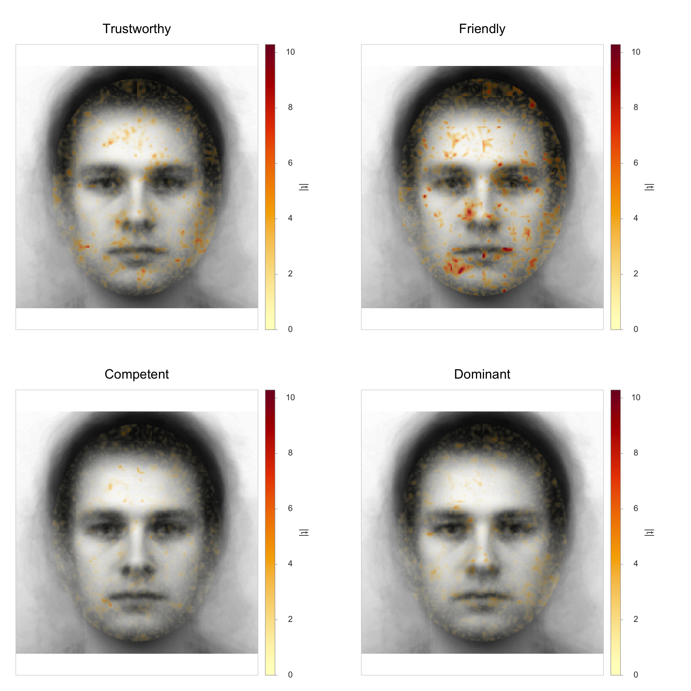
Within-condition producer agreement maps for the four warmth / agency traits, restricted to the full-face oval. Each panel overlays the per-pixel one-sample agreement statistic |t| on the male base face: pale yellow marks pixels where the 20 producers in that condition did not consistently push in one direction (low agreement); deep red marks pixels where they consistently pushed strongly in the same direction (high agreement). Pixels outside the face oval are fully transparent (background, hair edges, shoulders, image margin) so only in-face agreement is shown. The four panels share a common color scale (the same maximum in-face |t| across the four traits) so panel-to-panel intensity is comparable. The fire palette discards sign by design; for the signed view (which direction the agreement points), use plot_ci_overlay() or palette = diverging.

Among the four traits on this dataset, friendly and dominant show the broadest spread of red across the face; competent’s agreement map looks more diffuse, consistent with its weaker group-mean infoVal (§14.4) and its low per-region median z (§14.9).

15. Brief-RC end-to-end

The Brief-RC workflow follows the same diagnose, compute, and assess flow with two practical differences. First, the response data has multiple alternatives per trial (12 or 20, recorded as one row per trial carrying the chosen pool id and sign). Second, the noise matrix is consumed directly, without an rcicr wrapper.

15.1 Brief-RC variants currently supported

ci_from_responses_briefrc() accepts two method values, both matching the variants validated in Schmitz, Rougier, & Yzerbyt (2024):

• "briefrc12" (default): 12 alternatives per trial, 6 original + 6 inverted, arranged in a 3 x 4 grid in the Schmitz et al. study.
• "briefrc20": 20 alternatives per trial, 10 original + 10 inverted, arranged in a 4 x 5 grid in the Schmitz et al. study.

The CI computation is identical for both variants. Schmitz’s genMask() formula does not depend on how many alternatives are shown per trial; it always reduces to mean-by-stim of the chosen pool ids, divided by length(unique(chosen_stim)). The package’s random-responder reference simulator for infoval() similarly relies on a 50/50 original/inverted marginal per trial, which holds for any symmetric Brief-RC split. The method argument is therefore metadata: it is recorded in the result list (as $method) so that downstream code, reports, and citations can indicate which paradigm produced the data, but it does not branch the computation.

Other split sizes (Brief-RC 4, 6, 8, 10) are mentioned in the Schmitz et al. (2024) discussion as possible future variants worth investigating, but they have not been validated and are not exposed in rcisignal. If you genuinely need to compute masks for one of those configurations, the §14.5 hand-rolled five-step recipe applies unchanged (the formula is symmetric in the per-trial split), but the result should be reported as exploratory.

15.2 End-to-end Brief-RC example

library(rcisignal)

# 1. Read the Schmitz et al. 2024 noise matrix directly. You
#    can also generate your own pool with rcicr (one-off,
#    slow); read_noise_matrix() handles both.
nm <- read_noise_matrix("schmitz/noise_matrix.txt")

# 2. Diagnostics on Brief-RC responses.
report <- run_diagnostics(
  briefrc_responses,
  method       = "briefrc",
  noise_matrix = nm,
  expected_n   = 60L,
  base_image    = "base.jpg",
  infoval_iter = 1000L
)
report

# 3. Compute individual masks.
res <- ci_from_responses_briefrc(
  briefrc_responses,
  noise_matrix = nm,
  method       = "briefrc12",
  scaling      = "none"           # base_image not needed at scaling = "none"
)
signal <- res$signal_matrix

# 4. Reliability assessment (same metrics, same calls).
run_reliability(signal, seed = 1L)

# 5. Per-producer infoVal with trial-count-matched reference.
# Pass the same trial-level data frame: infoval derives the
# per-producer trial counts via table(responses$participant_id).
infoval(signal, nm,
        responses = briefrc_responses,
        iter      = 1000L, seed = 1L)

# 6. Save rendered CIs to PNG (visualization only). Do not
#    feed these to rel_* or to hand-rolled infoVal.
res_render <- ci_from_responses_briefrc(
  briefrc_responses,
  noise_matrix = nm,
  base_image   = "base.jpg",   # required when scaling != "none"
  scaling      = "matched"     # Schmitz Experiment 2 convention
)
# res_render$rendered_ci is base + matched(mask), ready for PNG

16. Caveats and reporting notes

A summary of what to keep in mind when reporting results.

Reliability and validity address different questions. The metrics in this package quantify whether a CI is stable (within-condition) and separable (between-condition). Whether the CI accurately reflects the producer’s mental representation of the target trait is a separate validity question, typically addressed by an external rater study or a behavioral validation, and the package does not address it. High rel_* values support claims about consistency and discriminability; plan validity work alongside the rcisignal pipeline.

Raw vs rendered. Pre-rendered PNGs are convenient and carry the scaling step into your pixel data. Variance-based metrics break under any scaling; correlation-based metrics survive a single uniform scaling and break under per-CI “matched” scaling. The package errors at runtime when a known-rendered matrix is fed to a variance-based metric. The cleanest workflow computes CIs from raw responses (ci_from_responses_*), feeds the returned $signal_matrix to all metrics, and renders to PNG only for visualization.

Group-mean z and per-producer z carry different information. Per-producer Frobenius norms aggregate over the whole image and dilute localised signal, so individual z values are systematically lower than group-mean z even when the group CI is highly informative (the §14.4 pattern). Report both, with the per-producer distribution (median z, % above 1.96) as the primary group-level summary per Brinkman et al. (2019) and the group-mean z as a supplementary headline number. The full reasoning — including a side-by-side simulation of the two reference distributions — is in §11.

FWER scope. rel_cluster_test() controls FWER across pixels within a single comparison. run_discriminability_pairwise() adds a second layer of FWER control across the K-choose-2 pair comparisons (Holm by default). Don’t double-correct: within-pair cluster p-values are already adjusted; the across-pairs Holm operates on the per-pair minimum cluster p.

Apply masks symmetrically. When infoval() uses a mask, both the observed Frobenius norm and the reference distribution are restricted to the same pixels. Other functions follow the same discipline. Mixing masked observed with unmasked reference (or vice versa) yields a number with no defensible interpretation.

Sample size. Reliability estimates themselves become unreliable below N approximately 30 per condition. The package warns at N < 30 and aborts at N < 4. Aim for N >= 60 per condition for stable assessment.

A bootstrap CI on a distance is not a test against zero. The Euclidean distance from rel_dissimilarity() (and the matrices behind plot_ci_distance_matrix() / plot_ci_mds()) is a non-negative norm whose bootstrap CI is biased upward by producer resampling and almost always excludes zero even when two conditions do not differ. Read it as a precision interval and for relative magnitude comparisons, not as evidence of a difference. For an above-chance test, set null = "permutation" and read d_z, d_ratio, and a permutation p against the positive-centred permutation null. The Pearson r fields carry the mirror-image bias (resampling attenuates r, so its CI sits below the observed value). See §9.3.

Many-condition summary figures. plot_ci_distance_matrix() and plot_ci_mds() share the same baseline-aware framing as rel_dissimilarity(): prefer Euclidean magnitude over absolute Pearson r for similarity claims, and report the per-k Kruskal stress trace from plot_ci_mds() alongside any 2D paper panel so readers can audit how much the projection is hiding. A 2D MDS map with stress > 0.10 should be read for relative ordering of points rather than absolute distances.

Pre-1.0 status. The package is not yet at version 1.0; argument names and defaults may change between minor versions, particularly when a change makes a sharp edge less easy to cut yourself on. The release notes (news(package = "rcisignal")) list every breaking change.

17. Appendix: troubleshooting low or negative infoVal

This appendix expands on the brief interpretation note in §10. If you compute infoval() and find that most or all per-producer z-scores sit well below 1.96, sometimes negative, even though spot checks suggest producers are doing the task seriously, that is a common pattern rather than evidence of a data problem. Five reasons in roughly the order they tend to apply.

1. Frobenius norm is a global energy statistic. It sums squared pixel deviations across the entire image. Real internal representations are usually spatially sparse, concentrated in face features (eyes, mouth, jaw) rather than spanning the whole image grid. Pixels outside that region contribute noise of similar magnitude to the chance reference, and that noise dilutes the signal-bearing region in the global norm. A producer with strong, visually-obvious signal in the eyes can therefore have a Frobenius norm only marginally above the random reference. (See point 4 below for the practical countermeasure.)

2. The reference is strict because it lives in the same subspace. Both the observed mask and the reference are projections onto the same low-dimensional sinusoidal noise basis. The reference distribution has plenty of overall energy by construction, so the only way to clear z = 1.96 is to align signs with a specific subset of patterns more than chance.

3. Per-trial signal is small. Each 2IFC choice contributes a tiny signal increment relative to the per-trial noise amplitude. With 300 trials the SNR gain is sqrt(300) ~ 17x, but if per-trial signal is on the order of 5% of per-trial noise, post-aggregation effective SNR is barely visible to a global energy measure.

4. Without a face mask, infoVal counts background. make_face_mask() ships a parametric full-face oval that isolates the face region from background and hair. Applying it (infoval(..., mask = make_face_mask(c(256, 256)))) concentrates the norm on signal-bearing pixels and typically lifts z-scores noticeably. The convention of applying a full-face oval before computing pixel-wise CI metrics follows prior practice in social-face RC (e.g., Oliveira et al., 2019; Ratner et al., 2014; Schmitz, Rougier, & Yzerbyt, 2024).

5. Group-level CIs can show higher z than individual CIs, but the inflation is conditional, not structural. Two pieces of math feed into this, and both need stating. First, averaging N producer masks under independent-noise assumptions reduces noise variance by 1/N and the noise norm by 1/sqrt(N). So the group-mean CI of N producers each contributing T trials has noise comparable to a single producer with N x T trials (a 20-producer condition at 300 trials each gives an effective 6000-trial noise floor). Second, whether that noise reduction actually translates into a sqrt(N)-style increase in group-mean infoVal over the per-producer median depends on whether the producers’ signals are spatially aligned. If producers share a common spatial template, signal survives the averaging and the group-mean z grows roughly as sqrt(N) above the per-producer floor. If producer templates are idiosyncratic, averaging cancels signal as well as noise and the group-mean z stays modest. The Oliveira et al. (2019) reanalysis in §14.4 shows both regimes in the same dataset: friendly / unfriendly, where per-producer signal is broadly shared, land at group-mean z of roughly 15-18; incompetent / unintelligent, where alignment is weaker, sit near z = 2. The ratio group_z / per_producer_median is therefore not a fixed inflation factor; it is a joint readout of N, T, and producer alignment.

   Brinkman et al. (2019) only ever computed infoVal on individual CIs. They reported a mean per-producer infoVal of 3.9 (lab) and 2.9 (online), with 68% / 54% of producers individually exceeding 1.96 (Brinkman et al., 2019, p. 2070). For group-level use they propose applying the infoVal metric to individual CIs and inspecting the resulting distribution (specifically the proportion of participants whose individual CIs cleared the chance reference), which they describe as a way “to assess the proportion of participants that contributed to the group CI” (Brinkman et al., 2019, p. 2071). They do not explicitly rule out computing infoVal on the averaged noise pattern, but they do not endorse it either; the group-mean infoVal this package offers (group_mean_z(), called inside infoval_report()) is a package-level extension of the Brinkman recipe and has not been independently validated for social-face RC (see §1.2). The §14.4 worked example reports both numbers alongside; treat the group-mean z as a supplementary headline, not a replacement for the Brinkman-style per-producer distribution.

17.1 Diagnostic recipe

If a per-producer infoVal table looks worryingly low, work through these steps before reporting it:

sm <- res$signal_matrix

# Each producer in this study did 300 trials. Build a named
# integer vector with one entry per producer (the names match
# the column names of `sm`).
tc <- rep(300L, ncol(sm))
names(tc) <- colnames(sm)

# 1. Compare observed and reference norm distributions directly.
iv  <- infoval(sm, noise_matrix, tc, iter = 1000L, seed = 1L)
ref <- iv$reference[[as.character(tc[1])]]
cat(sprintf(
  "observed median = %.4f, reference median = %.4f, %% above = %+.1f%%\n",
  median(iv$norms), median(ref),
  100 * (median(iv$norms) - median(ref)) / median(ref)
))

# 2. Apply the face mask. Per-producer z usually rises.
fm        <- make_face_mask(c(256L, 256L))
iv_masked <- infoval(sm, noise_matrix, tc, mask = fm,
                     iter = 1000L, seed = 1L)
median(iv_masked$infoval)

# 3. Compute the group-mean CI's infoVal. We treat the group as
# a single "producer" whose trial count is the sum of the
# individual counts.
group <- matrix(rowMeans(sm), ncol = 1,
                dimnames = list(NULL, "group"))
tc_grp <- sum(tc)
names(tc_grp) <- "group"

iv_grp <- infoval(group, noise_matrix, tc_grp,
                  iter = 1000L, seed = 1L)
iv_grp$infoval                 # value depends on signal alignment;
                               # see paragraph 5 of §17

# 4. Sanity-check the chance baseline. A random-mask producer
# should give z ~ 0 within MAD noise. Build a fake producer's
# mask out of 300 random stimuli and 300 random +/-1 responses,
# the same way Step 3 of §14.5 builds a real one.
rnd_stim <- sample(ncol(noise_matrix), 300L, replace = TRUE)
rnd_resp <- sample(c(-1, 1),           300L, replace = TRUE)
random_mask <- (noise_matrix[, rnd_stim] %*% rnd_resp) / 300

# Put the random mask into a 1-column matrix named "rnd" and run
# infoval() on it.
rnd_signal <- matrix(random_mask, ncol = 1,
                     dimnames = list(NULL, "rnd"))
tc_rnd <- 300L
names(tc_rnd) <- "rnd"

iv_rand <- infoval(rnd_signal, noise_matrix, tc_rnd,
                   iter = 1000L, seed = 1L)
iv_rand$infoval                 # should be ~ 0 within MAD noise

17.2 What’s up with negative z-scores?

A negative z indicates that the observed mask carries less Frobenius energy than the chance reference. This is informative rather than a calibration error. A clearly negative z (say, below -2) on a producer who allegedly engaged with the task suggests they responded inconsistently, partly randomly, or with selection patterns that average toward zero. Cross-check rel_loo_z(), response-time distributions, and any other attention checks before drawing conclusions.

17.3 What to report

For a publishable summary we typically recommend two complementary statistics:

• The median per-producer infoVal z and the proportion of producers above z = 1.96, mirroring Brinkman et al.’s (2019) reporting choice.
• The group-mean CI’s infoVal z as a supplementary headline number. Under signal alignment this can be substantially larger than the per-producer median, with a sqrt(N)-style upper envelope; under weak alignment it stays close to per-producer values (paragraph 5 of §17 spells out why). This metric is a package-level extension and has not been independently validated for social-face RC (§1.2), so report it as exploratory rather than primary.

The two numbers answer different questions. The median tells you how informative a typical individual CI is; the group-mean z tells you how informative the condition’s average CI is.

18. Citation

if (requireNamespace("rcisignal", quietly = TRUE)) {
  print(citation("rcisignal"))
} else {
  message(
    "Install rcisignal to view its citation: ",
    "devtools::install() or ",
    "remotes::install_github(\"olivethree/rcisignal\")."
  )
}
#> To cite package 'rcisignal' in publications use:
#> 
#>   Oliveira, M. (2026). rcisignal: Quality checks for
#>   reverse-correlation data and classification images (Version 0.3.1) [R
#>   package]. Zenodo. https://doi.org/10.5281/zenodo.19961180
#> 
#> A BibTeX entry for LaTeX users is
#> 
#>   @Manual{,
#>     title = {rcisignal: Quality checks for reverse-correlation data and classification images},
#>     author = {Manuel Oliveira},
#>     year = {2026},
#>     note = {R package version 0.3.1},
#>     doi = {10.5281/zenodo.19961180},
#>     url = {https://doi.org/10.5281/zenodo.19961180},
#>   }

19. References

Brinkman, L., Goffin, S., van de Schoot, R., van Haren, N. E. M., Dotsch, R., & Aarts, H. (2019). Quantifying the informational value of classification images. Behavior Research Methods, 51(5), 2059-2073. https://doi.org/10.3758/s13428-019-01232-2

Brinkman, L., Todorov, A., & Dotsch, R. (2017). Visualising mental representations: A primer on noise-based reverse correlation in social psychology. European Review of Social Psychology, 28(1), 333-361. https://doi.org/10.1080/10463283.2017.1381469

Brown, W. (1910). Some experimental results in the correlation of mental abilities. British Journal of Psychology, 3(3), 296-322. https://doi.org/10.1111/j.2044-8295.1910.tb00207.x

Chauvin, A., Worsley, K. J., Schyns, P. G., Arguin, M., & Gosselin, F. (2005). Accurate statistical tests for smooth classification images. Journal of Vision, 5(9), 1. https://doi.org/10.1167/5.9.1

Cone, J., Brown-Iannuzzi, J. L., Lei, R., & Dotsch, R. (2021). Type I error is inflated in the two-phase reverse correlation procedure. Social Psychological and Personality Science, 12(5), 760-768. https://doi.org/10.1177/1948550620938616

Cook, R. D. (1977). Detection of influential observation in linear regression. Technometrics, 19(1), 15-18. https://doi.org/10.1080/00401706.1977.10489493

DeBruine, L. (2022). webmorphR: Reproducible stimuli. https://github.com/debruine/webmorphR

Dotsch, R. (2016, 2023). rcicr: Reverse-Correlation Image- Classification Toolbox. https://github.com/rdotsch/rcicr

Koo, T. K., & Li, M. Y. (2016). A guideline of selecting and reporting intraclass correlation coefficients for reliability research. Journal of Chiropractic Medicine, 15(2), 155-163. https://doi.org/10.1016/j.jcm.2016.02.012

Kruskal, J. B. (1964). Multidimensional scaling by optimizing goodness of fit to a nonmetric hypothesis. Psychometrika, 29(1), 1-27. https://doi.org/10.1007/BF02289565

Lundqvist, D., Flykt, A., & Öhman, A. (1998). Karolinska Directed Emotional Faces (KDEF) [Database record]. APA PsycTests. https://doi.org/10.1037/t27732-000

Maris, E., & Oostenveld, R. (2007). Nonparametric statistical testing of EEG- and MEG-data. Journal of Neuroscience Methods, 164(1), 177-190. https://doi.org/10.1016/j.jneumeth.2007.03.024

McGraw, K. O., & Wong, S. P. (1996). Forming inferences about some intraclass correlation coefficients. Psychological Methods, 1(1), 30-46. https://doi.org/10.1037/1082-989X.1.1.30

Nichols, T. E., & Holmes, A. P. (2002). Nonparametric permutation tests for functional neuroimaging: a primer with examples. Human Brain Mapping, 15(1), 1-25. https://doi.org/10.1002/hbm.1058

Oliveira, M., Garcia-Marques, T., Dotsch, R., & Garcia-Marques, L. (2019). Dominance and competence face to face: Dissociations obtained with a reverse correlation approach. European Journal of Social Psychology. https://doi.org/10.1002/ejsp.2569

Ratner, K. G., Dotsch, R., Wigboldus, D. H. J., van Knippenberg, A., & Amodio, D. M. (2014). Visualizing minimal ingroup and outgroup faces: implications for impressions, attitudes, and behavior. Journal of Personality and Social Psychology, 106(6), 897-911. https://doi.org/10.1037/a0036498

Schmitz, M., Rougier, M., & Yzerbyt, V. (2020). Comment on “Quantifying the informational value of classification images”: A miscomputation of the infoVal metric. Behavior Research Methods, 52(3), 1383-1386. https://doi.org/10.3758/s13428-019-01295-1

Schmitz, M., Rougier, M., Yzerbyt, V., Brinkman, L., & Dotsch, R. (2020). Erratum to: Comment on “Quantifying the informational value of classification images”: Miscomputation of infoVal metric was a minor issue and is now corrected. Behavior Research Methods, 52(4), 1800-1801. https://doi.org/10.3758/s13428-020-01367-7

Schmitz, M., Rougier, M., & Yzerbyt, V. (2024). Introducing the brief reverse correlation: an improved tool to assess visual representations. European Journal of Social Psychology. https://doi.org/10.1002/ejsp.3100

Shrout, P. E., & Fleiss, J. L. (1979). Intraclass correlations: uses in assessing rater reliability. Psychological Bulletin, 86(2), 420-428. https://doi.org/10.1037/0033-2909.86.2.420

Smith, S. M., & Nichols, T. E. (2009). Threshold-free cluster enhancement: addressing problems of smoothing, threshold dependence and localisation in cluster inference. NeuroImage, 44(1), 83-98. https://doi.org/10.1016/j.neuroimage.2008.03.061

Spearman, C. (1910). Correlation calculated from faulty data. British Journal of Psychology, 3(3), 271-295. https://doi.org/10.1111/j.2044-8295.1910.tb00206.x

Tukey, J. W. (1958). Bias and confidence in not-quite large samples [Abstract]. Annals of Mathematical Statistics, 29(2), 614. https://doi.org/10.1214/aoms/1177706647